In this challenge, try using vector shapes to mask raster images in a thrilling mash-up of asset types!

The post Video Tutorial: Beginning App Asset Design Part 2: Challenge: Vector Masks appeared first on Ray Wenderlich.

Review what you've learned about raster images, and prepare to learn about color.

The post Video Tutorial: Beginning App Asset Design Part 2: Conclusion appeared first on Ray Wenderlich.

Apple’s Core ML and Vision frameworks have launched developers into a brave new world of machine learning, with an explosion of exciting possibilities. Vision lets you detect and track faces, and Apple’s Machine Learning page provides ready-to-use models that detect objects and scenes, as well as NSLinguisticTagger for natural language processing. If you want to build your own model, try Apple’s new Turi Create to extend one of its pre-trained models with your data.

But if what you want to do needs something even more customized? Then, it’s time to dive into machine learning (ML), using one of the many frameworks from Google, Microsoft, Amazon or Berkeley. And, to make life even more exciting, you’ll need to pick up a new programming language and a new set of development tools.

In this Keras machine learning tutorial you’ll learn how to train a deep-learning convolutional neural network model, convert it to Core ML, and integrate it into an iOS app. You’ll learn some ML terminology, use some new tools, and pick up a bit of Python along the way.

The sample project uses ML’s Hello-World example — a model that classifies hand-written digits, trained on the MNIST dataset.

Let’s get started!

Why Use Keras?

An ML model involves a lot of complex code, manipulating arrays and matrices. But ML has been around for a long time, and researchers have created libraries that make it much easier for people like us to create ML models. Many of these are written in Python, although researchers also use R, SAS, MATLAB and other software. But you’ll probably find everything you need in the Python-based tools:

• scikit-learn provides an easy way to run many classical ML algorithms, such as linear regression and support vector machines. Our Beginning Machine Learning with scikit-learn tutorial (coming soon!) shows you how to train these.
• At the other end of the spectrum are PyTorch and Google’s TensorFlow, which give you greater control over the inner workings of your deep learning model.
• Microsoft’s CNTK and Berkeley’s Caffe are similar deep learning frameworks, which have Python APIs to access their C++ engines.

So where does Keras fit in? It’s a wrapper around TensorFlow and CNTK, with Amazon’s MXNet coming soon. (It also works with Theano, but the University of Montreal stopped working on this in September 2017.) It provides an easy-to-use API for building models that you can train on one backend, and deploy on another.

Another reason to use Keras, rather than directly using TensorFlow, is that coremltools includes a Keras converter, but not a TensorFlow converter — although a TensorFlow to CoreML converter and a MXNet to CoreML converter exist. And while Keras supports CNTK as a backend, coremltools only works for Keras + TensorFlow.

Getting Started

Download and unzip the starter folder: it contains a starter iOS app, where you’ll add the ML model and code to use it. It also contains a docker-keras folder, which contains this tutorial’s Jupyter notebook.

Setting Up Docker

Docker is a container platform that lets you deploy apps in customized environments — sort of like a virtual machine, but different. Installing Docker gives you access to a large number of ML resources, mostly distributed as interactive Jupyter notebooks in Docker images.

Download, install, and start Docker Community Edition for Mac. In Terminal, enter the following commands, one at a time:

cd <where you unzipped starter>/starter/docker-keras
docker build -t keras-mnist .
docker run --rm -it -p 8888:8888 -v $(pwd)/notebook:/workspace/notebook keras-mnist

This last command maps the Docker container’s notebook folder to the local notebook folder, so you’ll have access to files written by the notebook, even after you logout of the Docker server.

At the very end of the command output is a URL containing a token. It looks like this, but with a different token value:

http://0.0.0.0:8888/?token=7b189c8e200f49dcc33845d39101e8a0ab257db5f3b539a7

Paste this URL into a browser to login to the Docker container’s notebook server.

Open the notebook folder, then open keras_mnist.ipynb. Tap the Not Trusted button to change it to Trusted: this allows you to save changes you make to the notebook, as well as the model files, in the notebook folder.

ML in a Nutshell

Arthur Samuel defined machine learning as “the field of study that gives computers the ability to learn without being explicitly programmed”. You have data, which has some features that can be used to classify the data, or use it to make some prediction, but you don’t have an explicit formula for computing this, so you can’t write a program to do it. If you have “enough” data samples, you can train a computer model to recognize patterns in this data, then apply its learning to new data. It’s called supervised learning when you know the correct outcomes for all the training data: then the model just checks its predictions against the known outcomes, and adjusts itself to reduce error and increase accuracy. Unsupervised learning is beyond the scope of this tutorial.

Weights & Threshold

Say you want to choose a restaurant for dinner with a group of friends. Several factors influence your decision: dietary restrictions, access to public transport, price range, type of food, child-friendliness, etc. You assign a weight to each factor, to indicate its importance for your decision. Then, for each restaurant in your list of options, you assign a value for each factor, according to how well the restaurant satisfies that factor. You multiply each factor value by the factor’s weight, and add these up to get the weighted sum. The restaurant with the highest result is the best choice. Another way to use this model is to produce binary output: yes or no. You set a threshold value, and remove from your list any restaurant whose weighted sum falls below this threshold.

Training an ML Model

Coming up with the weights isn’t an easy job. But luckily you have a lot of data from previous dinners, including which restaurant was chosen, so you can train an ML model to compute weights that produce the same results, as closely as possible. Then you apply these computed weights to future decisions.

To train an ML model, you start with random weights, apply them to the training data, then compare the computed outputs with the known outputs to calculate the error. This is a multi-dimensional function that has a minimum value, and the goal of training is to determine the weights that get very close to this minimum. The weights also need to work on new data: if the error over a large set of validation data is higher than the error over the training data, then the model is overfitted — the weights work too well on the training data, indicating training has mistakenly detected some feature that doesn’t generalize to new data.

Stochastic Gradient Descent

To compute weights that reduce the error, you calculate the gradient of the error function at the current graph location, then adjust the weights to “step down” the slope. This is called gradient descent, and happens many times during a training session. For large datasets, using all the data to calculate the gradient takes a long time. Stochastic gradient descent (SGD) estimates the gradient from randomly selected mini-batches of training data — like taking a survey of voters ahead of election day: if your sample is representative of the whole dataset, then the survey results accurately predict the final results.

Optimizers

The error function is lumpy: you have to be careful not to step too far, or you might miss the minimum. Your step rate also needs to have enough momentum to push you out of any false minimum. ML researchers have put a lot of effort into devising optimization algorithms to do this. The current favorite is Adam (Adaptive Moment estimation), which combines the features of previous favorites RMSprop (Root Mean Square propagation) and AdaGrad (Adaptive Gradient algorithm).

Keras Code Time!

OK, the Docker container should be ready now: go back and follow the instructions to open the notebook. It’s time to write some Keras code!

Enter the following code in the keras_mnist.ipynb cell with the matching heading. When you finish entering the code in each cell, press Control-Enter to run it. An asterisk appears in the In [ ]: label while the code is running, then a number will appear, to show the order in which you ran the cells. Everything stays in memory while you’re logged in to the notebook. Every so often, tap the Save and Checkpoint button.

Import Utilities & Dependencies

Enter the following code, and run it to check the Keras version.

from __future__ import print_function
from matplotlib import pyplot as plt

import keras
from keras.datasets import mnist
from keras.models import Sequential
from keras.layers import Dense, Dropout, Flatten
from keras.layers import Conv2D, MaxPooling2D
from keras.utils import np_utils
from keras import backend as K

import coremltools
# coremltools supports Keras version 2.0.6
print('keras version ', keras.__version__)

__future__ is the compatibility layer between Python 2 and Python 3: Python 2 has a print command (no parentheses), but Python 3 requires a print() function. Importing print_function allows you to use print() statements in Python 2 code.

Keras uses the NumPy mathematics library to manipulate arrays and matrices. Matplotlib is a plotting library for NumPy: you’ll use it to inspect a training data item.

After importing keras, print its version: coremltools supports version 2.0.6, and will spew warnings if you use a higher version. Keras already has the MNIST dataset, so you import that. Then the next three lines import the model components. You import the NumPy utilities, and you give the backend a label with import backend as K: you’ll use it to check image_data_format.

Finally, you import coremltools, which you’ll use at the end of this notebook.

Load & Pre-Process Data

Training & Validation Data Sets

First, get your data! Enter the code below, and run it: downloading the data takes a little while.

(x_train, y_train), (x_val, y_val) = mnist.load_data()

This downloads data from https://s3.amazonaws.com/img-datasets/mnist.npz, shuffles the data items, and splits them between a training dataset and a validation dataset. Validation data helps to detect the problem of overfitting the model to the training data. The training step uses the trained parameters to compute outputs for the validation data. You’ll set callbacks to monitor validation loss and accuracy, to save the model that performs best on the validation data, and possibly stop early, if validation loss or accuracy fail to improve for too many epochs (repetitions).

Inspect x & y Data

When the download finishes, enter the following code in the next cell, and run it to see what you got.

# Inspect x data
print('x_train shape: ', x_train.shape)
# Displays (60000, 28, 28)
print(x_train.shape[0], 'training samples')
# Displays 60000 train samples
print('x_val shape: ', x_val.shape)
# Displays (10000, 28, 28)
print(x_val.shape[0], 'validation samples')
# Displays 10000 validation samples

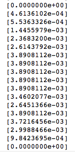
print('First x sample\n', x_train[0])
# Displays an array of 28 arrays, each containing 28 gray-scale values between 0 and 255
# Plot first x sample
plt.imshow(x_train[0])
plt.show()

# Inspect y data
print('y_train shape: ', y_train.shape)
# Displays (60000,)
print('First 10 y_train elements:', y_train[:10])
# Displays [5 0 4 1 9 2 1 3 1 4]

You have 60,000 28×28-pixel training samples and 10,000 validation samples. The first training sample is an array of 28 arrays, each containing 28 gray-scale values between 0 and 255. Looking at the non-zero values, you can see a shape like the digit 5.

Sure enough, the plt code shows the first training sample is a handwritten 5:

The y data is a 60000-element array containing the correct classifications of the training samples: the first training sample is 5, the next is 0, and so on.

Set Input & Output Dimensions

Enter these two lines, and run the cell to set up the basic dimensions of the x inputs and y outputs.

img_rows, img_cols = x_train.shape[1], x_train.shape[2]
num_classes = 10

MNIST data items are 28×28-pixel images, and you want to classify each as a digit between 0 and 9.

You use x_train.shape values to set the number of image rows and columns. x_train.shape is an array of 3 elements:

0. number of data samples: 60000
1. number of rows of each data sample: 28
2. number of columns of each data sample: 28

Reshape x Data & Set Input Shape

The model needs the data in a slightly different “shape”. Enter the code below, and run it.

# Set input_shape for channels_first or channels_last
if K.image_data_format() == 'channels_first':
    x_train = x_train.reshape(x_train.shape[0], 1, img_rows, img_cols)
    x_val = x_val.reshape(x_val.shape[0], 1, img_rows, img_cols)
    input_shape = (1, img_rows, img_cols)
else:
    x_train = x_train.reshape(x_train.shape[0], img_rows, img_cols, 1)
    x_val = x_val.reshape(x_val.shape[0], img_rows, img_cols, 1)
    input_shape = (img_rows, img_cols, 1)

Convolutional neural networks think of images as having width, height and depth. The depth dimension is called channels, and contains color information. Gray-scale images have 1 channel; RGB images have 3 channels.

Keras backends like TensorFlow and CNTK, expect image data in either channels-last format (rows, columns, channels) or channels-first format (channels, rows, columns). The reshape function inserts the channels in the correct position.

You also set the initial input_shape with the channels at the correct end.

Inspect Reshaped x Data

Enter the code below, and run it to see how the shapes have changed.

print('x_train shape:', x_train.shape)
# x_train shape: (60000, 28, 28, 1)
print('x_val shape:', x_val.shape)
# x_val shape: (10000, 28, 28, 1)
print('input_shape:', input_shape)
# input_shape: (28, 28, 1)

TensorFlow image data format is channels-last, so x_train.shape and x_val.shape now have a new element, 1, at the end.

Convert Data Type & Normalize Values

The model needs the data values in a specific format. Enter the code below, and run it.

x_train = x_train.astype('float32')
x_val = x_val.astype('float32')
x_train /= 255
x_val /= 255

MNIST image data values are of type uint8, in the range [0, 255], but Keras needs values of type float32, in the range [0, 1].

Inspect Normalized x Data

Enter the code below, and run it to see the changes to the x data.

print('First x sample, normalized\n', x_train[0])
# An array of 28 arrays, each containing 28 arrays, each with one value between 0 and 1

Now each value is an array, the values are floats, and the non-zero values are between 0 and 1.

Reformat y Data

The y data is a 60000-element array containing the correct classifications of the training samples, but it’s not obvious that there are only 10 categories. Enter the code below, and run it once only to reformat the y data.

print('y_train shape: ', y_train.shape)
# (60000,)
print('First 10 y_train elements:', y_train[:10])
# [5 0 4 1 9 2 1 3 1 4]
# Convert 1-dimensional class arrays to 10-dimensional class matrices
y_train = np_utils.to_categorical(y_train, num_classes)
y_val = np_utils.to_categorical(y_val, num_classes)
print('New y_train shape: ', y_train.shape)
# (60000, 10)

y_train is a 1-dimensional array, but the model needs a 60000 x 10 matrix to represent the 10 categories. You must also make the same conversion for the 10000-element y_val array.

Inspect Reformatted y Data

Enter the code below, and run it to see how the y data has changed.

print('New y_train shape: ', y_train.shape)
# (60000, 10)
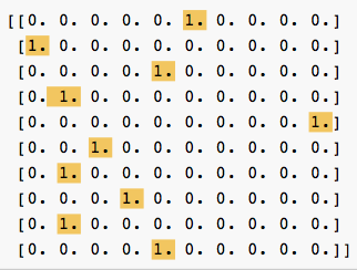
print('First 10 y_train elements, reshaped:\n', y_train[:10])
# An array of 10 arrays, each with 10 elements,
# all zeros except at index 5, 0, 4, 1, 9 etc.

y_train is now an array of 10-element arrays, each containing all zeros except at the index that the image matches.

Define Model Architecture

Model architecture is a form of alchemy, like secret family recipes for the perfect barbecue sauce or garam masala. You might start with a general-purpose architecture, then tweak it to exploit symmetries in your input data, or to produce a model with specific characteristics.

Here are models from two researchers: Sri Raghu Malireddi and François Chollet, the author of Keras. Chollet’s is general-purpose, and Malireddi’s is designed to produce a small model, suitable for mobile apps.

Enter the code below, and run it to see the model summaries.

Malireddi’s Architecture

model_m = Sequential()
model_m.add(Conv2D(32, (5, 5), input_shape=input_shape, activation='relu'))
model_m.add(MaxPooling2D(pool_size=(2, 2)))
model_m.add(Dropout(0.5))
model_m.add(Conv2D(64, (3, 3), activation='relu'))
model_m.add(MaxPooling2D(pool_size=(2, 2)))
model_m.add(Dropout(0.2))
model_m.add(Conv2D(128, (1, 1), activation='relu'))
model_m.add(MaxPooling2D(pool_size=(2, 2)))
model_m.add(Dropout(0.2))
model_m.add(Flatten())
model_m.add(Dense(128, activation='relu'))
model_m.add(Dense(num_classes, activation='softmax'))
# Inspect model's layers, output shapes, number of trainable parameters
print(model_m.summary())

Chollet’s Architecture

model_c = Sequential()
model_c.add(Conv2D(32, (3, 3), input_shape=input_shape, activation='relu'))
# Note: hwchong, elitedatascience use 32 for second Conv2D
model_c.add(Conv2D(64, (3, 3), activation='relu'))
model_c.add(MaxPooling2D(pool_size=(2, 2)))
model_c.add(Dropout(0.25))
model_c.add(Flatten())
model_c.add(Dense(128, activation='relu'))
model_c.add(Dropout(0.5))
model_c.add(Dense(num_classes, activation='softmax'))
# Inspect model's layers, output shapes, number of trainable parameters
print(model_c.summary())

Although Malireddi’s architecture has one more convolutional layer (Conv2D) than Chollet’s, it runs much faster, and the resulting model is much smaller.

Model Summaries

Take a quick look at the model summaries for these two models:

model_m:

Layer (type)                 Output Shape              Param #
=================================================================
conv2d_6 (Conv2D)            (None, 24, 24, 32)        832
_________________________________________________________________
max_pooling2d_5 (MaxPooling2 (None, 12, 12, 32)        0
_________________________________________________________________
dropout_6 (Dropout)          (None, 12, 12, 32)        0
_________________________________________________________________
conv2d_7 (Conv2D)            (None, 10, 10, 64)        18496
_________________________________________________________________
max_pooling2d_6 (MaxPooling2 (None, 5, 5, 64)          0
_________________________________________________________________
dropout_7 (Dropout)          (None, 5, 5, 64)          0
_________________________________________________________________
conv2d_8 (Conv2D)            (None, 5, 5, 128)         8320
_________________________________________________________________
max_pooling2d_7 (MaxPooling2 (None, 2, 2, 128)         0
_________________________________________________________________
dropout_8 (Dropout)          (None, 2, 2, 128)         0
_________________________________________________________________
flatten_3 (Flatten)          (None, 512)               0
_________________________________________________________________
dense_5 (Dense)              (None, 128)               65664
_________________________________________________________________
dense_6 (Dense)              (None, 10)                1290
=================================================================
Total params: 94,602
Trainable params: 94,602
Non-trainable params: 0

model_c:

Layer (type)                 Output Shape              Param #
=================================================================
conv2d_4 (Conv2D)            (None, 26, 26, 32)        320
_________________________________________________________________
conv2d_5 (Conv2D)            (None, 24, 24, 64)        18496
_________________________________________________________________
max_pooling2d_4 (MaxPooling2 (None, 12, 12, 64)        0
_________________________________________________________________
dropout_4 (Dropout)          (None, 12, 12, 64)        0
_________________________________________________________________
flatten_2 (Flatten)          (None, 9216)              0
_________________________________________________________________
dense_3 (Dense)              (None, 128)               1179776
_________________________________________________________________
dropout_5 (Dropout)          (None, 128)               0
_________________________________________________________________
dense_4 (Dense)              (None, 10)                1290
=================================================================
Total params: 1,199,882
Trainable params: 1,199,882
Non-trainable params: 0

The bottom line Total params is the main reason for the size difference: Chollet’s 1,199,882 is 12.5 times more than Malireddi’s 94,602. And that’s just about exactly the difference in model size: 4.8MB vs 380KB.

Malireddi’s model has three Conv2D layers, each followed by a MaxPooling2D layer, which halves the layer’s width and height. This makes the number of parameters for the first dense layer much smaller than Chollet’s, and explains why Malireddi’s model is much smaller and trains much faster. The implementation of convolutional layers is highly optimized, so the additional convolutional layer improves the accuracy without adding much to training time. But the smaller dense layer runs much faster than Chollet’s.

I’ll tell you about layers, output shape and parameter numbers in the Explanations section, while you wait for the next step to finish running.

Train the Model

Define Callbacks List

callbacks is an optional argument for the fit function, so define callbacks_list first.

Enter the code below, and run it.

callbacks_list = [
    keras.callbacks.ModelCheckpoint(
        filepath='best_model.{epoch:02d}-{val_loss:.2f}.h5',
        monitor='val_loss', save_best_only=True),
    keras.callbacks.EarlyStopping(monitor='acc', patience=1)
]

An epoch is a complete pass through all the mini-batches in the dataset.

The ModelCheckpoint callback monitors the validation loss value, saving the model with the lowest-so-far value in a file with the epoch number and the validation loss in the filename.

The EarlyStopping callback monitors training accuracy: if it fails to improve for two consecutive epochs, training stops early. In my experiments, this never happened: if acc went down in one epoch, it always recovered in the next.

Compile & Fit Model

Unless you have access to a GPU, I recommend you use Malireddi’s model_m for this step, as it runs much faster than Chollet’s model_c: on my MacBook Pro, 76-106s/epoch vs. 246-309s/epoch, or about 15 minutes vs. 45 minutes.

Enter the code below, and run it. This will take quite a while, so read the Explanations section while you wait. But check Finder after a couple of minutes, to make sure the notebook is saving .h5 files.

model_m.compile(loss='categorical_crossentropy',
                optimizer='adam', metrics=['accuracy'])

# Hyper-parameters
batch_size = 200
epochs = 10

# Enable validation to use ModelCheckpoint and EarlyStopping callbacks.
model_m.fit(
    x_train, y_train, batch_size=batch_size, epochs=epochs,
    callbacks=callbacks_list, validation_data=(x_val, y_val), verbose=1)

Convolutional Neural Network: Explanations

You can use just about any ML approach to create an MNIST classifier, but this tutorial uses a convolutional neural network (CNN), because that’s a key strength of TensorFlow and Keras.

Convolutional neural networks assume inputs are images, and arrange neurons in three dimensions: width, height, depth. A CNN consists of convolutional layers, each detecting higher-level features of the training images: the first layer might train filters to detect short lines or arcs at various angles; the second layer trains filters to detect significant combinations of these lines; the final layer’s filters build on the previous layers to classify the image.

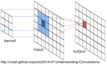
Each convolutional layer passes a small square kernel of weights — 1×1, 3×3 or 5×5 — over the input, computing the weighted sum of the input units under the kernel. This is the convolution process.

Each neuron is connected to only 1, 9, or 25 neurons in the previous layer, so there’s a danger of co-adapting — depending too much on a few inputs — and this can lead to overfitting. So CNNs include pooling and dropout layers to counteract co-adapting and overfitting. I explain these, below.

Sample Model

Here’s Malireddi’s model again:

model_m = Sequential()
model_m.add(Conv2D(32, (5, 5), input_shape=input_shape, activation='relu'))
model_m.add(MaxPooling2D(pool_size=(2, 2)))
model_m.add(Dropout(0.5))
model_m.add(Conv2D(64, (3, 3), activation='relu'))
model_m.add(MaxPooling2D(pool_size=(2, 2)))
model_m.add(Dropout(0.2))
model_m.add(Conv2D(128, (1, 1), activation='relu'))
model_m.add(MaxPooling2D(pool_size=(2, 2)))
model_m.add(Dropout(0.2))
model_m.add(Flatten())
model_m.add(Dense(128, activation='relu'))
model_m.add(Dense(num_classes, activation='softmax'))

Let’s work our way through this code.

Sequential

You first create an empty Sequential model, then add a linear stack of layers: the layers run in the sequence that they’re added to the model. The Keras documentation has several examples of Sequential models.

The first layer must have information about the input shape, which for MNIST is (28, 28, 1). The other layers infer their input shape from the output shape of the previous layer. Here’s the output shape part of the model summary:

Layer (type)                 Output Shape              Param #
=================================================================
conv2d_6 (Conv2D)            (None, 24, 24, 32)        832
_________________________________________________________________
max_pooling2d_5 (MaxPooling2 (None, 12, 12, 32)        0
_________________________________________________________________
dropout_6 (Dropout)          (None, 12, 12, 32)        0
_________________________________________________________________
conv2d_7 (Conv2D)            (None, 10, 10, 64)        18496
_________________________________________________________________
max_pooling2d_6 (MaxPooling2 (None, 5, 5, 64)          0
_________________________________________________________________
dropout_7 (Dropout)          (None, 5, 5, 64)          0
_________________________________________________________________
conv2d_8 (Conv2D)            (None, 5, 5, 128)         8320
_________________________________________________________________
max_pooling2d_7 (MaxPooling2 (None, 2, 2, 128)         0
_________________________________________________________________
dropout_8 (Dropout)          (None, 2, 2, 128)         0
_________________________________________________________________
flatten_3 (Flatten)          (None, 512)               0
_________________________________________________________________
dense_5 (Dense)              (None, 128)               65664
_________________________________________________________________
dense_6 (Dense)              (None, 10)                1290

Conv2D

This model has three Conv2D layers:

Conv2D(32, (5, 5), input_shape=input_shape, activation='relu')
Conv2D(64, (3, 3), activation='relu')
Conv2D(128, (1, 1), activation='relu')

• The first parameter — 32, 64, 128 — is the number of filters, or features, you want to train this layer to detect. This is also the depth — the last dimension — of the output shape.
• The second parameter — (5, 5), (3, 3), (1, 1) — is the kernel size: a tuple specifying the width and height of the convolution window that slides over the input space, computing weighted sums — dot products of the kernel weights and the input unit values.
• The third parameter activation='relu' specifies the ReLU (Rectified Linear Unit) activation function. When the kernel is centered on an input unit, the unit is said to activate or fire if the weighted sum is greater than a threshold value: weighted_sum > threshold. The bias value is -threshold: the unit fires if weighted_sum + bias > 0. Training the model calculates the kernel weights and the bias value for each filter. ReLU is the most popular activation function for deep neural networks.

MaxPooling2D

MaxPooling2D(pool_size=(2, 2))

A pooling layer slides an n-rows by m-columns filter across the previous layer, replacing the n x m values with their maximum value. Pooling filters are usually square: n = m. The most commonly used 2 x 2 pooling filter, shown below, halves the width and height of the previous layer, thus reducing the number of parameters, which helps control overfitting.

Malireddi’s model has a pooling layer after each convolutional layer, which greatly reduces the final model size and training time.

Chollet’s model has two convolutional layers before pooling. This is recommended for larger networks, as it allows the convolutional layers to develop more complex features before pooling discards 75% of the values.

Conv2D and MaxPooling2D parameters determine each layer’s output shape and number of trainable parameters:

Output Shape = (input width – kernel width + 1, input height – kernel height + 1, number of filters)

You can’t center a 3×3 kernel over the first and last units in each row and column, so the output width and height are 2 pixels less than the input. A 5×5 kernel reduces output width and height by 4 pixels.

• Conv2D(32, (5, 5), input_shape=(28, 28, 1)): (28-4, 28-4, 32) = (24, 24, 32)
• MaxPooling2D halves the input width and height: (24/2, 24/2, 32) = (12, 12, 32)
• Conv2D(64, (3, 3)): (12-2, 12-2, 64) = (10, 10, 64)
• MaxPooling2D halves the input width and height: (10/2, 10/2, 64) = (5, 5, 64)
• Conv2D(128, (1, 1)): (5-0, 5-0, 128) = (5, 5, 128)

Param # = number of filters x (kernel width x kernel height x input depth + 1 bias)

• Conv2D(32, (5, 5), input_shape=(28, 28, 1)): 32 x (5x5x1 + 1) = 832
• Conv2D(64, (3, 3)): 64 x (3x3x32 + 1) = 18,496
• Conv2D(128, (1, 1)): 128 x (1x1x64 + 1) = 8320

Challenge: Calculate the output shapes and parameter numbers for Chollet’s architecture model_c.

Dropout

Dropout(0.5)
Dropout(0.2)

A dropout layer is often paired with a pooling layer. It randomly sets a fraction of input units to 0. This is another method to control overfitting: neurons are less likely to be influenced too much by neighboring neurons, because any of them might drop out of the network at random. This makes the network less sensitive to small variations in the input, so more likely to generalize to new inputs.

Aurélien Géron, in Hands-on Machine Learning with Scikit-Learn & TensorFlow, compares this to a workplace where, on any given day, some percentage of the people might not come to work: everyone would have to be able to do critical tasks, and would have to cooperate with more co-workers. This would make the company more resilient, and less dependent on any single worker.

Flatten

The weights from the convolutional layers must be made 1-dimensional — flattened — before passing them to the fully connected Dense layer.

model_m.add(Dropout(0.2))
model_m.add(Flatten())
model_m.add(Dense(128, activation='relu'))

The output shape of the previous layer is (2, 2, 128), so the output of Flatten() is an array with 512 elements.

Dense

Dense(128, activation='relu')
Dense(num_classes, activation='softmax')

Each neuron in a convolutional layer uses the values of only a few neurons in the previous layer. Each neuron in a fully connected layer uses the values of all the neurons in the previous layer. The Keras name for this type of layer is Dense.

Looking at the model summaries above, Malireddi’s first Dense layer has 512 neurons, while Chollet’s has 9216. Both produce a 128-neuron output layer, but Chollet’s must compute 18 times more parameters than Malireddi’s. This is what uses most of the additional training time.

Most CNN architectures end with one or more Dense layers and then the output layer.

The first parameter is the output size of the layer. The final output layer has an output size of 10, corresponding to the 10 classes of digits.

The softmax activation function produces a probability distribution over the 10 output classes. It’s a generalization of the sigmoid function, which scales its input value into the range [0, 1]. For your MNIST classifier, softmax scales each of 10 values into [0, 1], such that they add up to 1.

You would use the sigmoid function for a single output class: for example, what’s the probability that this is a photo of a good dog?

Compile

model_m.compile(loss='categorical_crossentropy', optimizer='adam', metrics=['accuracy'])

The categorical crossentropy loss function measures the distance between the probability distribution calculated by the CNN, and the true distribution of the labels.

An optimizer is the stochastic gradient descent algorithm that tries to minimize the loss function by following the gradient down at just the right speed.

Accuracy — the fraction of the images that were correctly classified — is the most common metric monitored during training and testing.

Fit

batch_size = 256
epochs = 10
model_m.fit(x_train, y_train, batch_size=batch_size, epochs=epochs, callbacks=callbacks_list,
            validation_data=(x_val, y_val), verbose=1)

Batch size is the number of data items to use for mini-batch stochastic gradient fitting. Choosing a batch size is a matter of trial and error, a roll of the dice. Smaller values make epochs take longer; larger values make better use of GPU parallelism, and reduce data transfer time, but too large might cause you to run out of memory.

The number of epochs is also a roll of the dice. Each epoch should improve loss and accuracy measurements. More epochs should produce a more accurate model, but training takes longer. Too many epochs can result in overfitting. You set up a callback to stop early, if the model stops improving before completing all the epochs. In the notebook, you can re-run the fit cell to keep improving the model.

When you loaded the data, 10000 items were set as validation data. Passing this argument enables validation while training, so you can monitor validation loss and accuracy. If these values are worse than the training loss and accuracy, this indicates that the model is overfitted.

Verbose

0 = silent, 1 = progress bar, 2 = one line per epoch.

Results

Here’s the result of one of my training runs:

Epoch 1/10
60000/60000 [==============================] - 106s - loss: 0.0284 - acc: 0.9909 - val_loss: 0.0216 - val_acc: 0.9940
Epoch 2/10
60000/60000 [==============================] - 100s - loss: 0.0271 - acc: 0.9911 - val_loss: 0.0199 - val_acc: 0.9942
Epoch 3/10
60000/60000 [==============================] - 102s - loss: 0.0260 - acc: 0.9914 - val_loss: 0.0228 - val_acc: 0.9931
Epoch 4/10
60000/60000 [==============================] - 101s - loss: 0.0257 - acc: 0.9913 - val_loss: 0.0211 - val_acc: 0.9935
Epoch 5/10
60000/60000 [==============================] - 101s - loss: 0.0256 - acc: 0.9916 - val_loss: 0.0222 - val_acc: 0.9928
Epoch 6/10
60000/60000 [==============================] - 100s - loss: 0.0263 - acc: 0.9913 - val_loss: 0.0178 - val_acc: 0.9950
Epoch 7/10
60000/60000 [==============================] - 87s - loss: 0.0231 - acc: 0.9920 - val_loss: 0.0212 - val_acc: 0.9932
Epoch 8/10
60000/60000 [==============================] - 76s - loss: 0.0240 - acc: 0.9922 - val_loss: 0.0212 - val_acc: 0.9935
Epoch 9/10
60000/60000 [==============================] - 76s - loss: 0.0261 - acc: 0.9916 - val_loss: 0.0220 - val_acc: 0.9934
Epoch 10/10
60000/60000 [==============================] - 76s - loss: 0.0231 - acc: 0.9925 - val_loss: 0.0203 - val_acc: 0.9935

With each epoch, loss values should decrease, and accuracy values should increase. The ModelCheckpoint callback saves epochs 1, 2 and 6, because validation loss values in epochs 3, 4 and 5 are higher than epoch 2’s, and there’s no improvement in validation loss after epoch 6. Training doesn’t stop early, because training accuracy never decreases for two consecutive epochs.

By now, your model has finished training, so back to coding!

Convert to Core ML Model

When the training step is complete, you should have a few models saved in notebook. The one with the highest epoch number (and lowest validation loss) is the best model, so use that filename in the convert function.

Enter the following code, and run it.

output_labels = ['0', '1', '2', '3', '4', '5', '6', '7', '8', '9']
# For the first argument, use the filename of the newest .h5 file in the notebook folder.
coreml_mnist = coremltools.converters.keras.convert(
    'best_model.09-0.03.h5', input_names=['image'], output_names=['output'],
    class_labels=output_labels, image_input_names='image')

Here, you set the 10 output labels in an array, and pass this as the class_labels argument. If you train a model with a lot of output classes, put the labels in a text file, one label per line, and set the class_labels argument to the file name.

In the parameter list, you supply input and output names, and set image_input_names='image' so the Core ML model accepts an image as input, instead of a multi-array.

Inspect Core ML model

Enter this line, and run it to see the printout.

print(coreml_mnist)

Just check that the input type is imageType, not multi-array:

input {
  name: "image"
  shortDescription: "Digit image"
  type {
    imageType {
      width: 28
      height: 28
      colorSpace: GRAYSCALE
    }
  }
}

Add Metadata for Xcode

Now add the following, substituting your own name and license info for the first two items, and run it.

coreml_mnist.author = 'raywenderlich.com'
coreml_mnist.license = 'Razeware'
coreml_mnist.short_description = 'Image based digit recognition (MNIST)'
coreml_mnist.input_description['image'] = 'Digit image'
coreml_mnist.output_description['output'] = 'Probability of each digit'
coreml_mnist.output_description['classLabel'] = 'Labels of digits'

This information appears when you select the model in Xcode’s Project navigator.

Save the Core ML Model

Finally, add the following, and run it.

coreml_mnist.save('MNISTClassifier.mlmodel')

This saves the mlmodel file in the notebook folder.

Congratulations, you now have a Core ML model that classifies handwritten digits! It’s time to use it in the iOS app.

Use Model in iOS App

Now you just follow the procedure described in Core ML and Vision: Machine Learning in iOS 11 Tutorial. The steps are the same, but I’ve rearranged the code to match Apple’s sample app Image Classification with Vision and CoreML.

Step 1. Drag the model into the app:

Open the starter app in Xcode, and drag MNISTClassifier.mlmodel from Finder into the project’s Project navigator. Select it to see the metadata you added:

If instead of Automatically generated Swift model class it says to build the project to generate the model class, go ahead and do that.

Step 2. Import the CoreML and Vision frameworks:

Open ViewController.swift, and import the two frameworks, just below import UIKit:

import CoreML
import Vision

Step 3. Create VNCoreMLModel and VNCoreMLRequest objects:

Add the following code below the outlets:

lazy var classificationRequest: VNCoreMLRequest = {
  // Load the ML model through its generated class and create a Vision request for it.
  do {
    let model = try VNCoreMLModel(for: MNISTClassifier().model)
    return VNCoreMLRequest(model: model, completionHandler: handleClassification)
  } catch {
    fatalError("Can't load Vision ML model: \(error).")
  }
}()

func handleClassification(request: VNRequest, error: Error?) {
  guard let observations = request.results as? [VNClassificationObservation]
    else { fatalError("Unexpected result type from VNCoreMLRequest.") }
  guard let best = observations.first
    else { fatalError("Can't get best result.") }

  DispatchQueue.main.async {
    self.predictLabel.text = best.identifier
    self.predictLabel.isHidden = false
  }
}

The request object works for any image that the handler in Step 4 passes to it, so you only need to define it once, as a lazy var.

The request object’s completion handler receives request and error objects. You check that request.results is an array of VNClassificationObservation objects, which is what the Vision framework returns when the Core ML model is a classifier, rather than a predictor or image processor.

A VNClassificationObservation object has two properties: identifier — a String — and confidence — a number between 0 and 1 — the probability the classification is correct. You take the first result, which will have the highest confidence value, and dispatch back to the main queue to update predictLabel. Classification work happens off the main queue, because it can be slow.

Step 4. Create and run a VNImageRequestHandler:

Locate predictTapped(), and replace the print statement with the following code:

let ciImage = CIImage(cgImage: inputImage)
let handler = VNImageRequestHandler(ciImage: ciImage)
do {
  try handler.perform([classificationRequest])
} catch {
  print(error)
}

You create a CIImage from inputImage, then create the VNImageRequestHandler object for this ciImage, and run the handler on an array of VNCoreMLRequest objects — in this case, just the one request object you created in Step 3.

Build and run. Draw a digit in the center of the drawing area, then tap Predict. Tap Clear to try again.

Larger drawings tend to work better, but the model often has trouble with ‘7’ and ‘4’. Not surprising, as a PCA visualization of the MNIST data shows 7s and 4s clustered with 9s:

Thanks to Sri Raghu M, Matthijs Hollemans and Hon Weng Chong for helpful discussions!

Where To Go From Here?

You can download the complete notebook and project for this tutorial here. If the model shows up as missing in the app, replace it with the one in the notebook folder.

You’re now well-equipped to train a deep learning model in Keras, and integrate it into your app. Here are some resources and further reading to deepen your own learning:

Resources

• Keras Documentation
• coremltools.converters.keras.convert
• Matthijs Hollemans’s blog
• Jason Brownlee’s blog

Further Reading

• François Chollet, Deep Learning with Python, Manning Publications
• Stanford CS231N Convolutional Networks
• Comparing Top Deep Learning Frameworks
• Preprocessing in Data Science (Part 1): Centering, Scaling, and KNN
• Gentle Introduction to the Adam Optimization Algorithm for Deep Learning

I hope you enjoyed this introduction to machine learning and Keras. Please join the discussion below if you have any questions or comments.

The post Beginning Machine Learning with Keras & Core ML appeared first on Ray Wenderlich.

Find out what we'll be covering in the final part of the course, focusing on color and image file formats.

The post Video Tutorial: Beginning App Asset Design Part 3: Introduction appeared first on Ray Wenderlich.

Welcome to the Swift Dojo! Learn about a really cool practice to help you improve your skills as a Swift developer: Swift Code Katas!

The post Screencast: Swift Code Katas: Introduction appeared first on Ray Wenderlich.

Grab a helmet for this crash course in color theory, and gain some perspective on how to think about color in your app.

The post Video Tutorial: Beginning App Asset Design Part 3: Working with Color appeared first on Ray Wenderlich.

Practice analyzing contrast between text and its background with the help of a web contrast checker.

The post Video Tutorial: Beginning App Asset Design Part 3: Challenge: Contrast and Accessibility appeared first on Ray Wenderlich.

Blueprints is a very popular way to create gameplay in Unreal Engine 4. However, if you’re a long-time programmer and prefer sticking to code, C++ is for you! Using C++, you can also make changes to the engine and also make your own plugins.

In this tutorial, you will learn how to:

• Create C++ classes
• Add components and make them visible to Blueprints
• Create a Blueprint class based on a C++ class
• Add variables and make them editable in Blueprints
• Bind axis and action mappings to functions
• Override C++ functions in Blueprints
• Bind an overlap event to a function

Please note that this is not a tutorial on learning C++. Instead, this tutorial will focus on working with C++ in the context of Unreal Engine.

Getting Started

If you haven’t already, you will need to install Visual Studio. Follow Epic’s official guide on setting up Visual Studio for Unreal Engine 4. (Although you can use alternative IDEs, this tutorial will use Visual Studio as Unreal is already designed to work with it.)

Afterwards, download the starter project and unzip it. Navigate to the project folder and open CoinCollector.uproject. If it asks you to rebuild modules, click Yes.

Once that is done, you will see the following scene:

In this tutorial, you will create a ball that the player will control to collect coins. In previous tutorials, you have been creating player-controlled characters using Blueprints. For this tutorial, you will create one using C++.

Creating a C++ Class

To create a C++ class, go to the Content Browser and select Add New\New C++ Class.

This will bring up the C++ Class Wizard. First, you need to select which class to inherit from. Since the class needs to be player-controlled, you will need a Pawn. Select Pawn and click Next.

In the next screen, you can specify the name and path for your .h and .cpp files. Change Name to BasePlayer and then click Create Class.

This will create your files and then compile your project. After compiling, Unreal will open Visual Studio. If BasePlayer.cpp and BasePlayer.h are not open, go to the Solution Explorer and open them. You can find them under Games\CoinCollector\Source\CoinCollector.

Before we move on, you should know about Unreal’s reflection system. This system powers various parts of the engine such as the Details panel and garbage collection. When you create a class using the C++ Class Wizard, Unreal will put three lines into your header:

1. #include "TypeName.generated.h"
2. UCLASS()
3. GENERATED_BODY()

Unreal requires these lines in order for a class to be visible to the reflection system. If this sounds confusing, don’t worry. Just know that the reflection system will allow you to do things such as expose functions and variables to Blueprints and the editor.

You’ll also notice that your class is named ABasePlayer instead of BasePlayer. When creating an actor-type class, Unreal will prefix the class name with A (for actor). The reflection system requires classes to have the appropriate prefixes in order to work. You can read about the other prefixes in Epic’s Coding Standard.

That’s all you need to know about the reflection system for now. Next, you will add a player model and camera. To do this, you need to use components.

Adding Components

For the player Pawn, you will add three components:

1. Static Mesh: This will allow you to select a mesh to represent the player
2. Spring Arm: This component operates like a camera boom. One end will be attached to the mesh and the camera will be attached to the other end.
3. Camera: Whatever this camera sees is what Unreal will display to the player

First, you need to include headers for each type of component. Open BasePlayer.h and then add the following lines above #include "BasePlayer.generated.h":

#include "Components/StaticMeshComponent.h"
#include "GameFramework/SpringArmComponent.h"
#include "Camera/CameraComponent.h"

#include "CoreMinimal.h"
#include "GameFramework/Pawn.h"
#include "Components/StaticMeshComponent.h"
#include "GameFramework/SpringArmComponent.h"
#include "Camera/CameraComponent.h"
#include "BasePlayer.generated.h"

Now you need to declare variables for each component. Add the following lines after SetupPlayerInputComponent():

UStaticMeshComponent* Mesh;
USpringArmComponent* SpringArm;
UCameraComponent* Camera;

The name you use here will be the name of the component in the editor. In this case, the components will display as Mesh, SpringArm and Camera.

Next, you need to make each variable visible to the reflection system. To do this, add UPROPERTY() above each variable. Your code should now look like this:

UPROPERTY()
UStaticMeshComponent* Mesh;

UPROPERTY()
USpringArmComponent* SpringArm;

UPROPERTY()
UCameraComponent* Camera;

You can also add specifiers to UPROPERTY(). These will control how the variable behaves with various aspects of the engine.

Add VisibleAnywhere and BlueprintReadOnly inside the brackets for each UPROPERTY(). Separate each specifier with a comma.

UPROPERTY(VisibleAnywhere, BlueprintReadOnly)

VisibleAnywhere will allow each component to be visible within the editor (including Blueprints).

BlueprintReadOnly will allow you to get a reference to the component using Blueprint nodes. However, it will not allow you to set the component. It is important for components to be read-only because their variables are pointers. You do not want to allow users to set this otherwise they could point to a random location in memory. Note that BlueprintReadOnly will still allow you to set variables inside of the component, which is the desired behavior.

Now that you have variables for each component, you need to initialize them. To do this, you must create them within the constructor.

Initializing Components

To create components, you can use CreateDefaultSubobject<Type>("InternalName"). Open BasePlayer.cpp and add the following lines inside ABasePlayer():

Mesh = CreateDefaultSubobject<UStaticMeshComponent>("Mesh");
SpringArm = CreateDefaultSubobject<USpringArmComponent>("SpringArm");
Camera = CreateDefaultSubobject<UCameraComponent>("Camera");

This will create a component of each type. It will then assign their memory address to the provided variable. The string argument will be the component’s internal name used by the engine (not the display name although they are the same in this case).

Next you need to set up the hierarchy (which component is the root and so on). Add the following after the previous code:

RootComponent = Mesh;
SpringArm->SetupAttachment(Mesh);
Camera->SetupAttachment(SpringArm);

The first line will make Mesh the root component. The second line will attach SpringArm to Mesh. Finally, the third line will attach Camera to SpringArm.

Now that the component code is complete, you need to compile. Perform one of the following methods to compile:

1. In Visual Studio, select Build\Build Solution
2. In Unreal Engine, click Compile in the Toolbar

Next, you need to set which mesh to use and the rotation of the spring arm. It is advisable to do this in Blueprints because you do not want to hard-code asset paths in C++. For example, in C++, you would need to do something like this to set a static mesh:

static ConstructorHelpers::FObjectFinder<UStaticMesh> MeshToUse(TEXT("StaticMesh'/Game/MyMesh.MyMesh");
MeshComponent->SetStaticMesh(MeshToUse.Object);

However, in Blueprints, you can just select a mesh from a drop-down list.

If you were to move the asset to another folder, your Blueprints wouldn’t break. However, in C++, you would have to change every reference to that asset.

To set the mesh and spring arm rotation within Blueprints, you will need to create a Blueprint based on BasePlayer.

Subclassing C++ Classes

In Unreal Engine, navigate to the Blueprints folder and create a Blueprint Class. Expand the All Classes section and search for BasePlayer. Select BasePlayer and then click Select.

Rename it to BP_Player and then open it.

First, you will set the mesh. Select the Mesh component and set its Static Mesh to SM_Sphere.

Next, you need to set the spring arm’s rotation and length. This will be a top-down game so the camera needs to be above the player.

Select the SpringArm component and set Rotation to (0, -50, 0). This will rotate the spring arm so that the camera points down towards the mesh.

Since the spring arm is a child of the mesh, it will start spinning when the ball starts spinning.

To fix this, you need to set the rotation of the spring arm to be absolute. Click the arrow next to Rotation and select World.

Afterwards, set Target Arm Length to 1000. This will place the camera 1000 units away from the mesh.

Next, you need to set the Default Pawn Class in order to use your Pawn. Click Compile and then go back to the editor. Open the World Settings and set Default Pawn to BP_Player.

Press Play to see your Pawn in the game.

The next step is to add functions so the player can move around.

Implementing Movement

Instead of adding an offset to move around, you will move around using physics! First, you need a variable to indicate how much force to apply to the ball.

Go back to Visual Studio and open BasePlayer.h. Add the following after the component variables:

UPROPERTY(EditAnywhere, BlueprintReadWrite)
float MovementForce;

EditAnywhere allows you to edit MovementForce in the Details panel. BlueprintReadWrite will allow you to set and read MovementForce using Blueprint nodes.

Next, you will create two functions. One for moving up and down and another for moving left and right.

Creating Movement Functions

Add the following function declarations below MovementForce:

void MoveUp(float Value);
void MoveRight(float Value);

Later on, you will bind axis mapppings to these functions. By doing this, axis mappings will be able to pass in their scale (which is why the functions need the float Value parameter).

Now, you need to create an implementation for each function. Open BasePlayer.cpp and add the following at the end of the file:

void ABasePlayer::MoveUp(float Value)
{
	FVector ForceToAdd = FVector(1, 0, 0) * MovementForce * Value;
	Mesh->AddForce(ForceToAdd);
}

void ABasePlayer::MoveRight(float Value)
{
	FVector ForceToAdd = FVector(0, 1, 0) * MovementForce * Value;
	Mesh->AddForce(ForceToAdd);
}

MoveUp() will add a physics force on the X-axis to Mesh. The strength of the force is provided by MovementForce. By multiplying the result by Value (the axis mapping scale), the mesh can move in either the positive or negative directions.

MoveRight() does the same as MoveUp() but on the Y-axis.

Now that the movement functions are complete, you need to bind the axis mappings to them.

Binding Axis Mappings to Functions

For the sake of simplicity, I have already created the axis mappings for you. You can find them in the Project Settings under Input.

Add the following inside SetupPlayerInputComponent():

InputComponent->BindAxis("MoveUp", this, &ABasePlayer::MoveUp);
InputComponent->BindAxis("MoveRight", this, &ABasePlayer::MoveRight);

This will bind the MoveUp and MoveRight axis mappings to MoveUp() and MoveRight().

That’s it for the movement functions. Next, you need to enable physics on the Mesh component.

Enabling Physics

Add the following lines inside ABasePlayer():

Mesh->SetSimulatePhysics(true);
MovementForce = 100000;

The first line will allow physics forces to affect Mesh. The second line will set MovementForce to 100,000. This means 100,000 units of force will be added to the ball when moving. By default, physics objects weigh about 110 kilograms so you need a lot of force to move them!

If you’ve created a subclass, some properties won’t change even if you’ve changed it within the base class. In this case, BP_Player won’t have Simulate Physics enabled. However, any subclasses you create now will have it enabled by default.

Compile and then go back to Unreal Engine. Open BP_Player and select the Mesh component. Afterwards, enable Simulate Physics.

Click Compile and then press Play. Use W, A, S and D to move around.

Next, you will declare a C++ function that you can implement using Blueprints. This allows designers to create functionality without having to use C++. To learn this, you will create a jump function.

Creating the Jump Function

First you need to bind the jump mapping to a function. In this tutorial, jump is set to space bar.

Go back to Visual Studio and open BasePlayer.h. Add the following below MoveRight():

UPROPERTY(EditAnywhere, BlueprintReadWrite)
float JumpImpulse;

UFUNCTION(BlueprintImplementableEvent)
void Jump();

First is a float variable called JumpImpulse. You will use this when implementing the jump. It uses EditAnywhere to make it editable within the editor. It also uses BlueprintReadWrite so you can read and write it using Blueprint nodes.

Next is the jump function. UFUNCTION() will make Jump() visible to the reflection system. BlueprintImplementableEvent will allow Blueprints to implement Jump(). If there is no implementation, any calls to Jump() will do nothing.

Since Jump is an action mapping, the method to bind it is slightly different. Close BasePlayer.h and then open BasePlayer.cpp. Add the following inside SetupPlayerInputComponent():

InputComponent->BindAction("Jump", IE_Pressed, this, &ABasePlayer::Jump);

This will bind the Jump mapping to Jump(). It will only execute when you press the jump key. If you want it to execute when the key is released, use IE_Released instead.

Up next is overriding Jump() in Blueprints.

Overriding Functions in Blueprints

Compile and then close BasePlayer.cpp. Afterwards, go back to Unreal Engine and open BP_Player. Go to the My Blueprints panel and hover over Functions to display the Override drop-down. Click it and select Jump. This will create an Event Jump.

Next, create the following setup:

This will add an impulse (JumpImpulse) on the Z-axis to Mesh. Note that in this implementation, the player can jump indefinitely.

Next, you need to set the value of JumpImpulse. Click Class Defaults in the Toolbar and then go to the Details panel. Set JumpImpulse to 100000.

Click Compile and then close BP_Player. Press Play and jump around using space bar.

In the next section, you will make the coins disappear when the player touches them.

Collecting Coins

To handle overlaps, you need to bind a function to an overlap event. To do this, the function must meet two requirements. The first is that the function must have the UFUNCTION() macro. The second requirement is the function must have the correct signature. In this tutorial, you will use the OnActorBeginOverlap event. This event requires a function to have the following signature:

FunctionName(AActor* OverlappedActor, AActor* OtherActor)

Go back to Visual Studio and open BaseCoin.h. Add the following below PlayCustomDeath():

UFUNCTION()
void OnOverlap(AActor* OverlappedActor, AActor* OtherActor);

After binding, OnOverlap() will execute when the coin overlaps another actor. OverlappedActor will be the coin and OtherActor will be the other actor.

Next, you need to implement OnOverlap().

Implementing Overlaps

Open BaseCoin.cpp and add the following at the end of the file:

void ABaseCoin::OnOverlap(AActor* OverlappedActor, AActor* OtherActor)
{
}

Since you only want to detect overlaps with the player, you need to cast OtherActor to ABasePlayer. Before you do the cast, you need to include the header for ABasePlayer. Add the following below #include "BaseCoin.h":

#include "BasePlayer.h"

Now you need to perform the cast. In Unreal Engine, you can cast like this:

Cast<TypeToCastTo>(ObjectToCast);

If the cast is successful, it will return a pointer to ObjectToCast. If unsuccessful, it will return nullptr. By checking if the result is nullptr, you can determine if the object was of the correct type.

Add the following inside OnOverlap():

if (Cast<ABasePlayer>(OtherActor) != nullptr)
{
	Destroy();
}

Now, when OnOverlap() executes, it will check if OtherActor is of type ABasePlayer. If it is, destroy the coin.

Next, you need to bind OnOverlap().

Binding the Overlap Function

To bind a function to an overlap event, you need to use AddDynamic() on the event. Add the following inside ABaseCoin():

OnActorBeginOverlap.AddDynamic(this, &ABaseCoin::OnOverlap);

This will bind OnOverlap() to the OnActorBeginOverlap event. This event occurs whenever this actor overlaps another actor.

Compile and then go back to Unreal Engine. Press Play and start collecting coins. When you overlap a coin, the coin will destroy itself, causing it to disappear.

In the next section, you will create another overridable C++ function. However, this time you will also create a default implementation. To demonstrate this, you will use OnOverlap().

Creating a Function’s Default Implementation

To make a function with a default implementation, you need to use the BlueprintNativeEvent specifier. Go back to Visual Studio and open BaseCoin.h. Add BlueprintNativeEvent to the UFUNCTION() of OnOverlap():

UFUNCTION(BlueprintNativeEvent)
void OnOverlap(AActor* OverlappedActor, AActor* OtherActor);

To make a function the default implementation, you need to add the _Implementation suffix. Open BaseCoin.cpp and change OnOverlap to OnOverlap_Implementation:

void ABaseCoin::OnOverlap_Implementation(AActor* OverlappedActor, AActor* OtherActor)

Now, if a child Blueprint does not implement OnOverlap(), this implementation will be used instead.

The next step is to implement OnOverlap() in BP_Coin.

Creating the Blueprint Implementation

For the Blueprint implementation, you will call PlayCustomDeath(). This C++ function will increase the coin’s rotation rate. After 0.5 seconds, the coin will destroy itself.

To call a C++ function from Blueprints, you need to use the BlueprintCallable specifier. Close BaseCoin.cpp and then open BaseCoin.h. Add the following above PlayCustomDeath():

UFUNCTION(BlueprintCallable)

Compile and then close Visual Studio. Go back to Unreal Engine and open BP_Coin. Override On Overlap and then create the following setup:

Now whenever a player overlaps a coin, Play Custom Death will execute.

Click Compile and then close BP_Coin. Press Play and collect some coins to test the new implementation.

Where to Go From Here?

You can download the completed project here.

As you can see, working with C++ in Unreal Engine is quite easy. Although you’ve accomplished a lot so far with C++, there is still a lot to learn! I’d recommend checking out Epic’s tutorial series on creating a top-down shooter using C++.

If you’re new to Unreal Engine, check out our 10-part beginner series. This series will take you through various systems such as Blueprints, Materials and Particle Systems.

If there’s a topic you’d like me to cover, let me know in the comments below!

The post Unreal Engine 4 C++ Tutorial appeared first on Ray Wenderlich.

In this tutorial, you are going to learn how to accept credit cards in an iOS app using an amazing service called Stripe. You will walk through the whole process, from creating your Stripe account to accepting customer payments.

Stripe is an easy way to accept online and mobile app payments from both individuals and businesses.

There are two main features provided by the Stripe service. First of all, it avoids all the bureaucracy of creating a merchant account while still ensuring transaction safety. Also, it allows you to set up a developer account without verifying any business information. You can start accepting credit cards with Stripe’s API after signing up using the test environment. Moving to production is easy. All you need to do is to switch out your test API keys with live ones, and that’s it!

Getting Started: Creating Your Stripe Account

The first step is to get your API keys from Stripe. Head over to stripe.com and click on the green button that says CREATE ACCOUNT. Notice the phrase The new standard in online payments is stamped right on the homepage. So far, so good!

At this point, you are going to create a full-fledged Stripe account. It does not require to have your business details handy since we are going to use test data.

Insert your details (don’t forget to check the Captcha box) and click Create your Stripe account. You will be greeted with a dialog to add a mobile recovery number. If you chose not to do so now, click Skip.

To find your keys, click on API on the dashboard’s left menu.

As shown below, Stripe generates a pair of test secret/publishable API keys for your account. You won’t be able to use your live keys until you verify your account with Stripe. For the purposes of this tutorial, and whenever you’re just developing, you want to use the test secret and test publishable keys.

RWPuppies: The Stripe Sample Project

Your project for this tutorial is RWPuppies, a fully-functional mobile storefront that sells and ships puppies right to your door and accepts payments using credit cards. Full disclosure: This app will not ship puppies right to your door. Sorry if that’s a disappointment!

The app consists of the following three tabs:

• Featured Puppy: Displays the puppy of the day. This tab contains the puppy’s detailed information like name, breed and price. There’s even an Add to Cart button right there on the view controller if you decide to buy the featured pup on a whim. :]
• Inventory: Displays the entire list of puppies on sale in table format. Tapping on any cell takes you to that pup’s details page, which looks very similar to the featured puppy page.
• Checkout: Shows all the puppies that are currently in your cart, along with a running total for your order. Tapping on Continue takes you to a view controller where you can enter your credit card information and complete your purchase.

You don’t want to waste your time setting up table views or dragging out buttons in Interface Builder when you’re here to learn about Stripe so you’ll be happy to hear this tutorial provides you with a starter project that has everything unrelated to Stripe already implemented for you.

You can download the starter project here.

Open RWPuppies.xcworkspace. Build and run RWPuppies to give it a whirl, and notice that the UI and most of the functionality is already in place.

Real-world e-commerce apps typically get their inventory data from a remote server. For simplicity, the ten puppies on display, including the featured puppy, are all read from a local file named puppies.json. The contents look something like this:

[

{
 "id" : 12252012,
 "name" : "Penny",
 "breed" : "Dachshund",
 "photo_large" : "http://www.raywenderlich.com/downloads/puppies/dachshund.jpeg",
 "cuddle_factor" : 5,
 "price" : 29999
 },

 ...
]

The checkout cart is implemented as a singleton called CheckoutCart. You can add and remove any number of puppies to and from your cart and all the changes will be reflected automatically in the third tab, which contains your order information.

Your primary task is to integrate the logic to collect and send the payment to your simple back-end app that will talk to Stripe.

“But I’m a mobile developer. I don’t do back end!” Fear not. You’ll find it’s pretty straightforward. :]

Time To Earn Your Stripes

The sequence of steps leading to a successful credit card charge looks like this:

1. The app sends your customer’s credit card information to Stripe using a secure HTTPS POST request. The only required bits of information you need to send to Stripe are the credit card number, the expiration month and the expiration year. Not even the owner’s name is required!

   Sending additional information, such as the card’s CVC number and billing address, is not required but is highly recommended. This extra information helps reduce fraudulent transactions that the merchant (that means you or your client) have to cover.

2. Stripe processes the credit card information and returns a one-time token to your app. Getting this token from Stripe does not mean that your customer’s card was charged. The actual charge is initiated later from your server.
3. Assuming the previous step was successful, your app posts the one-time token to your server for the grand finale.
4. Server-side, you must contact Stripe again using Stripe’s API. Luckily for you, the fine folks at Stripe have provided official libraries in several popular languages that wrap around their underlying HTTP API. You’ll be using Sinatra-based web application for this tutorial.
5. Stripe’s servers attempt to charge the credit card and send the result, success or failure, back to your server.
6. In the last step of what seems to be an endless game of telephone, your server notifies your iOS app of the transaction’s final result.

Getting Acquainted With Stripe’s iOS Library

There are different ways to add Stripe’s library. According to Stripe’s iOS Integration documentation, they support CocoaPods, Carthage, both Static and Dynamic Frameworks, as well as Fabric.

The starter project uses CocoaPods. In order to not lose the focus of this tutorial, all the dependencies have been set up for you. You don’t need to run any CocoaPod commands!

Now it’s time to start coding! You start by implementing the code for steps 1 and 2 above: submitting the credit card information to Stripe and getting a token.

Open Constants.swift. You will find an enum with a few constants. The first one is for the publishable API key that you got from Stripe when you signed up for an account.

Replace the value of publishableKey with your Test Publishable Key. It should be a random string of numbers and letters that starts with pk_test.

Ignore the baseURLString for now. You’ll get to that later.

Open AppDelegate.swift and at the top of the file, add the import below:

import Stripe

Next, replace the existing definition of application(_:didFinishLaunchingWithOptions:) with this:

func application(_ application: UIApplication,
                 didFinishLaunchingWithOptions launchOptions: [UIApplicationLaunchOptionsKey: Any]?)
                 -> Bool {
  STPPaymentConfiguration.shared().publishableKey = Constants.publishableKey
  return true
}

Here you are configuring Stripe with your publishable key.

Now, your next step is to collect credit card details from the user.

Accepting Credit Cards

At the moment, tapping on the Continue button on the checkout view controller does nothing. Open CheckoutViewController.swift and add this import just below the existing UIKit import at the top:

import Stripe

Then, complete the definition of continueDidTap(_:) Interface Builder action with this:

// 1
guard CheckoutCart.shared.canPay else {
  let alertController = UIAlertController(title: "Warning",
                                          message: "Your cart is empty",
                                          preferredStyle: .alert)
  let alertAction = UIAlertAction(title: "OK", style: .default)
  alertController.addAction(alertAction)
  present(alertController, animated: true)
  return
}
// 2
let addCardViewController = STPAddCardViewController()
addCardViewController.delegate = self
navigationController?.pushViewController(addCardViewController, animated: true)

If you build at this point, you’ll find a compilation error. Don’t worry about it; you’ll solve it in the next step.
Here’s what happening in the code above:

1. Ensure the user has placed at least one puppy in the checkout cart. If not, show a warning message and return.
2. Create an instance of STPAddCardViewController, set its delegate and present it to the user.

STPAddCardViewController is a view controller class included in Stripe’s framework. It handles both collecting and tokenizing the user’s payment information. Once presented, the user will see a screen to input the credit card details like the number, expiration date and CVC.

Since our checkout view controller has been set as a delegate of STPAddCardViewController, you must implement the required methods. In CheckoutViewController.swift, add the following code at the end of the file:

extension CheckoutViewController: STPAddCardViewControllerDelegate {

  func addCardViewControllerDidCancel(_ addCardViewController: STPAddCardViewController) {
    navigationController?.popViewController(animated: true)
  }

  func addCardViewController(_ addCardViewController: STPAddCardViewController,
                             didCreateToken token: STPToken,
                             completion: @escaping STPErrorBlock) {
  }
}

You’ve added two different methods.

• addCardViewControllerDidCancel(_:) is called when the user cancels adding a card.
• addCardViewController(_:didCreateToken:completion:) is called when the user successfully adds a card and your app receives a token from Stripe.

Next, it’s time to finish the StripeClient component. It’s a singleton class that interacts with your back end.

Open StripeClient.swift. As usual, import Stripe module at the top of the file:

import Stripe

Now, add the following method:

func completeCharge(with token: STPToken, amount: Int, completion: @escaping (Result) -> Void) {
  // 1
  let url = baseURL.appendingPathComponent("charge")
  // 2
  let params: [String: Any] = [
    "token": token.tokenId,
    "amount": amount,
    "currency": Constants.defaultCurrency,
    "description": Constants.defaultDescription
  ]
  // 3
  Alamofire.request(url, method: .post, parameters: params)
    .validate(statusCode: 200..<300)
    .responseString { response in
      switch response.result {
      case .success:
        completion(Result.success)
      case .failure(let error):
        completion(Result.failure(error))
      }
  }
}

Here's the breakdown of the above code:

1. First, append the charge method path to the baseURL, in order to invoke the charge API available in your back end. You will implement this API shortly.

2. Next, build a dictionary containing the parameters needed for the charge API. token, amount and currency are mandatory fields.

   The amount is an Int since Stripe API deals only with cents. When displaying amount values, your iOS app uses a currency number formatter.

3. Finally, make a network request using Alamofire to perform the charge. When the request completes, it invokes a completion closure with the result of the request.

Open CheckoutViewController.swift and locate addCardViewController(_:didCreateToken:completion:). Add the following code to it:

StripeClient.shared.completeCharge(with: token, amount: CheckoutCart.shared.total) { result in
  switch result {
  // 1
  case .success:
    completion(nil)

    let alertController = UIAlertController(title: "Congrats",
                          message: "Your payment was successful!",
                          preferredStyle: .alert)
    let alertAction = UIAlertAction(title: "OK", style: .default, handler: { _ in
      self.navigationController?.popViewController(animated: true)
    })
    alertController.addAction(alertAction)
    self.present(alertController, animated: true)
  // 2
  case .failure(let error):
    completion(error)
  }
}

This code calls completeCharge(with:amount:completion:) and when it receives the result:

1. If the Stripe client returns with a success result, it calls completion(nil) to inform STPAddCardViewController the request was successful and then presents a message to the user.
2. If the Stripe client returns with a failure result, it simply calls completion(error) letting STPAddCardViewController handle the error since it has internal logic for this.

Build what you've got so far to make sure everything’s implemented correctly.

Well done! Now it's time to set up the back-end script that is going to complete the credit card payment.

Setting Up Your Ruby Back End

Setting up a back-end development environment is beyond the scope of this tutorial, so you'll keep it as simple as possible. The back end is going to be a Sinatra web application that expects you to send the token id returned by STPAddCardViewController, along with a few other parameters.

Sinatra requires a Ruby environment greater or equal to 1.9.3. In order to check the version currently installed in your machine, open Terminal and paste the following command:

ruby --version

You should get something like:

ruby 2.4.0p0 (2016-12-24 revision 57164) [x86_64-darwin16]

If you have an older version, you need to update it to the latest. The best way to install a new Ruby version is through RVM, a command line utility tool which allows you to easily install, manage, and work with multiple Ruby environments from interpreters to sets of gems.

In Terminal, paste the following command:

curl -sSL https://get.rvm.io | bash -s stable --ruby

Run ruby --version again. Now you should have all set up correctly.

At this point, you can install the Stripe, Sinatra and JSON gems.

Switch again to the Terminal and copy the following line:

gem install stripe sinatra json

Here you are instructing Ruby to install three gems into the current Ruby version. If you update your Ruby version, you'll need to repeat this process.

That's it! Now you are able to create your back end.

The Ruby Script

Open your favorite text editor (like Atom or TextEdit) and create a new file.

Paste the following code and save it as web.rb:

#1
require 'sinatra'
require 'stripe'
require 'json'

#2
Stripe.api_key = 'YOUR_TEST_SECRET_KEY'

#3
get '/' do
  status 200
  return "RWPuppies back end has been set up correctly"
end

#4
post '/charge' do
  #5
  payload = params
  if request.content_type.include? 'application/json' and params.empty?
    payload = indifferent_params(JSON.parse(request.body.read))
  end

  begin
    #6
    charge = Stripe::Charge.create(
      :amount => payload[:amount],
      :currency => payload[:currency],
      :source => payload[:token],
      :description => payload[:description]
    )
    #7
    rescue Stripe::StripeError => e
    status 402
    return "Error creating charge: #{e.message}"
  end
  #8
  status 200
  return "Charge successfully created"

end

Following the numbered comments, here’s what this code does:

1. First, you import several modules the script is going to need.

   Your app's request is going to arrive in JSON format, so you need to import the json module to be able to convert the incoming request into a proper dictionary.

2. Here, you need to replace YOUR_TEST_SECRET_KEY with your Test Secret Key that Stripe provided earlier. This is the secret part of the secret/publishable pair of keys necessary to complete a transaction. If there is a mismatch between the secret and publishable keys, the charge will fail.
3. Create the base / route that will print RWPuppies back end has been set up correctly if the back end has been set up correctly. You'll use this to test your server.
4. Create /charge route. It will listen for requests from the iOS app and send charge requests to Stripe.
5. Parse the JSON sent by your iOS application.
6. Create and invoke Stripe::Charge with various POST parameters.
   • amount: The amount in cents that you’ll charge your customer. You don't need to make any conversion here since your iOS app deals already with cents.
   • currency: A short string that identifies the currency used for the transaction. Its value has been set to usd within your iOS app.
   • source: The one-time token that you get back from STPAddCardViewControllerDelegate.
   • description: A descriptive message that you can easily recognize when you log into the Stripe dashboard. This is a good place for an internal transaction ID.
7. Keep in mind that errors can occur here as well. For example, you might try to charge a token that you already used. Whatever the outcome, you have to notify your app of what happened. You do this by returning the response that you receive from Stripe.
8. If everything goes as planned, your Stripe account should have more $$. :]

Save the file and try to run the script you've just created.

Go back to Terminal and paste the following command:

ruby web.rb

You should see something like this:

== Sinatra (v2.0.0) has taken the stage on 4567 for development with backup from Thin

The back end is launched and listening for requests in the port 4567. Open your favorite web browser and type http://localhost:4567 in your address bar. You should see something like this:

Back To Your App

With your back end in place, it’s time to test your application.

Only one little thing is missing. You need to configure the back end URL in the application. As you've just seen, your back end runs locally as a Sinatra web application.

Open Constants.swift file and find the static variable called baseURLString. Replace the placeholder string with http://localhost:4567. Your code should look like the following:

enum Constants {
  static let publishableKey = "pk_test_FGACeszCTD2vvtx3rm5xr8rB"
  static let baseURLString = "http://localhost:4567"
  static let defaultCurrency = "usd"
  static let defaultDescription = "Purchase from RWPuppies iOS"
}

defaultCurrency and defaultDescription are set respectively to usd and Purchase from RWPuppies iOS. Obviously in a real world app those values should not be hardcoded but based on customers' information.

Now, build and run. Go through the entire checkout process. Add one or more favorites puppies to your cart and open the Checkout tab. At this point you should be able to see the list of the puppies you are going to buy and the total amount.

Click Continue. Insert the following card details into the credit card view:

• Credit Card Number: 4242424242424242
• Expiration Date: Any month and year in the future
• CVC Number: Any three or four-digit number

Tap the Done button in the top right corner. If the payment succeeded, you will get something like the following:

More importantly, verify that the charge went through Stripe. Open your Stripe dashboard and go straight to Payments on the left menu. You will find an entry similar to the one below.

Congratulations!

Where To Go From Here?

You've successfully implemented Stripe checkout in iOS from start to finish and your app can now accept credit cards. Whenever you want to start charging your customers, verify your Stripe account and switch all the test API keys to the live API keys.

Here are the finished iOS project and finished server script.

There are lots of cool things you can do with Stripe's API that this tutorial didn’t cover. For example, if you know you are going to be charging the same person in the future, you may want to create a customer object. If you need to collect shipping details, you can do that as well. Stripe also lets you create subscription plans and invoices if that suits your business model. Furthermore, in live mode, Stripe lets you to send email to charged customers for payment recaps.

I encourage you to peruse Stripe's docs if you're interested in implementing any of the features I mentioned above. If you have any tips or suggestions for using Stripe with iOS, or if you’ve implemented a checkout cart in the past, please share in the comments section.

The post Accepting Credit Cards In Your iOS App Using Stripe appeared first on Ray Wenderlich.

We often get emails from students who say they would love to attend RWDevCon, but can’t afford it on a Ramen-budget. Trust me, we’ve been there! :]

So today, we are happy to announce some exciting news – we are offering 5 student scholarships for RWDevCon 2018.

The 5 lucky students will win a free ticket to the conference and are invited to attend our team-only pre-conference fun day.

Attending RWDevCon 2018 is an amazing opportunity for students – through two days packed full of high quality hands-on tutorials, you’ll bring your iOS development skills up-to-date, learn a ton, and have a blast.

Keep reading to find out who’s eligible, how to apply, and who to thank for this great opportunity!

Eligibility and How To Apply

To be eligible to win, there are three requirements:

• You must be enrolled in a full-time educational program (such as high school, college/university, or a full-time immersive boot camp).
• You also must be able to attend the conference and the pre-conference fun day (Apr 5 – April 7, 2018).
• You must be able to pay for your own travel and hotel expenses (they are not included; the scholarship includes a ticket to the conference and an invitation to the team-only pre-conference fun day only).

Applying is simple:

• Just send us an email about why you’re interested in programming and why you’d like to attend RWDevCon. Please include proof that you are in a full-time educational program (a scanned ID or receipt is fine).

Applications are due in 2 weeks – February 22, 2018 – so apply now! :]

Last year’s student scholarship winners!

Introducing the Patrons

The RWDevCon 2018 scholarships are sponsored by 5 generous patrons of the iOS community, who bought a special ticket that included the cost of the student tickets.

I asked each of our patrons to write some advice for students studying programming. Here’s what they had to say:

Where To Go From Here?

If you, or a student you know, wants to take advantage of an amazing learning opportunity that will pay some major dividends in life, don’t miss this chance!

Just send us an email about why you’re interested in programming and why you’d like to attend RWDevCon. Please include proof that you are in a full-time educational program (a scanned ID or receipt is fine).

We wish the best of luck to all of the applicants, and we look forward to seeing you at RWDevCon 2018!

The post RWDevCon 2018 Student Scholarships: Apply Now! appeared first on Ray Wenderlich.

Android runs on a wide variety of devices that offer different screen sizes and densities. Because of this, it is important for Android apps to have a responsive user interface that can adapt to these different screens. Since the early days of the Android platform, system APIs have provided very powerful abstractions to design adaptive UIs, also known as adaptive layouts.

This is an update to our adaptive UI in Android tutorial which will show you how to build apps that work across different devices by dealing with the fragmentation in the Android device market. You’ll learn about:

• Configuration qualifiers
• Alternative layouts and drawables
• And layout previews in Android Studio — an immensely useful tool

What would a tutorial be without something to tinker with? It’d be pretty boring. So, you’ll build the user interface for a simple weather app completely from scratch! When you’re done, the screen will display an image, text labels and a map in three different configurations. Apps look so cool and well built when they have an adaptive UI. :]

Getting Started

Download the starter project named Adaptive Weather here, and open it in Android Studio 3.0.1 or later. Then build and run.

The app displays a simple RecyclerView listing several cities.

To learn all about RecyclerViews, we recommend reading our Android RecyclerView tutorial.

Open the build.gradle file of the app module to declare the following dependency:

dependencies {
  ...
  implementation 'com.google.android:flexbox:0.3.2'
}

Google’s FlexBox provides an implementation of the FlexBox specification on the Android platform. As you will see later on, it is a very useful tool for designing adaptive layouts. And combining it with Android’s resource qualifier system makes it even more powerful!

During this tutorial, you’ll often switch between the Android and Project modes in the Project navigator. Generally speaking:

• Android mode is the default when working within Android Studio because it provides a clean and simple file structure.
• Project mode is also necessary for building alternative layouts.

Weather Icons

Android devices have different screen densities, and for that reason it’s a good practice to import static images in multiple sizes. This is one way Android’s system APIs provide a way to create adaptive UIs. As described in the Supporting Multiple Screens guide, the categories of screen densities are:

• ldpi (low) ~120dpi
• mdpi (medium) ~160dpi
• hdpi (high) ~240dpi
• xhdpi (extra-high) ~320dpi
• xxhdpi (extra-extra-high) ~480dpi
• xxxhdpi (extra-extra-extra-high) ~640dpi

Whilst some UI editors make it easy to export images in different sizes, we will be exploring a different approach in this tutorial. Android Studio recently added support for Vector Drawables. This means that all your assets can be imported once and will be scaled at runtime depending on the device configuration (screen size and orientation).

Download the Weather Icons and extract. In Android Studio right-click on res/drawable and click on the New\Vector Asset menu item:

Select Local file (SVG, PSD) under Asset Type. From the filesystem location chooser under Path locate the weather-icons folder and choose the first icon, cloud.svg. Make sure to check the Override under Size setting otherwise your icons will look a bit distorted later on (¯\_(ツ)_/¯). Click Next and Finish:

Now you should see your icon in Android Studio as res/drawable/ic_cloud.xml. Repeat the same operations for the other icons: fog, rain, snow, sun, thunder.

Finally, enable the use of Vector Drawables in the app module’s build.gradle as follows:

android {
  ...

  defaultConfig {
      ...
      vectorDrawables.useSupportLibrary = true
  }
}

With scalable assets now in place in the project, you’re ready to start customizing the layouts.

Building layouts

With the dependencies declared, you get to shift your focus to building some layouts!

This simple application only contains one screen, which is represented by MainActivity. From the Project navigator, open res/layout/activity_main.xml. Click on the Preview button on the right side to see it in action.

An activity comprises a Kotlin or Java class — in this case MainActivity.kt — and a layout file. In fact, one activity can have several layouts, as you’ll see shortly. For now, it’s important to remember that the existing layout file, activity_main.xml, is the default layout.

Forecast Grid View

First, define the default layout for your main activity. To start this, open res/values/colors.xml and replace its content with the following:

<?xml version="1.0" encoding="utf-8"?>
<resources>
  <color name="color_primary">#9B26AF</color>
  <color name="color_primary_dark">#89229b</color>
  <color name="text_color_primary">#ffffff</color>
  <color name="forecast_grid_background">#89bef2</color>
</resources>

Here you’re overriding the default Material theme colors and providing a background color for the forecast grid. Next, right-click on the values folder and select the New\Value resource file menu:

Enter fractions.xml for the file name and paste the following:

<?xml version="1.0" encoding="utf-8"?>
<resources>
  <item name="weather_icon" type="fraction">33%</item>
</resources>

Here you’re specifying that the width taken by each icon should be 1/3 of the total width.

Next, create a new layout in res/layout called forecast_grid.xml and add the following list of images inside a FlexboxLayout:

<?xml version="1.0" encoding="utf-8"?>
<com.google.android.flexbox.FlexboxLayout xmlns:android="http://schemas.android.com/apk/res/android"
  xmlns:app="http://schemas.android.com/apk/res-auto"
  android:id="@+id/forecast"
  android:layout_width="match_parent"
  android:layout_height="match_parent"
  android:background="@color/forecast_grid_background"
  app:alignItems="center"
  app:flexWrap="wrap"
  app:justifyContent="space_around">

  <android.support.v7.widget.AppCompatImageView
    android:id="@+id/day1"
    android:layout_width="wrap_content"
    android:layout_height="60dp"
    app:layout_flexBasisPercent="@fraction/weather_icon"
    app:srcCompat="@drawable/ic_thunder" />

  <android.support.v7.widget.AppCompatImageView
    android:id="@+id/day2"
    android:layout_width="wrap_content"
    android:layout_height="60dp"
    app:layout_flexBasisPercent="@fraction/weather_icon"
    app:srcCompat="@drawable/ic_fog" />

  <android.support.v7.widget.AppCompatImageView
    android:id="@+id/day3"
    android:layout_width="wrap_content"
    android:layout_height="60dp"
    app:layout_flexBasisPercent="@fraction/weather_icon"
    app:srcCompat="@drawable/ic_rain" />

  <android.support.v7.widget.AppCompatImageView
    android:id="@+id/day4"
    android:layout_width="wrap_content"
    android:layout_height="60dp"
    app:layout_flexBasisPercent="@fraction/weather_icon"
    app:srcCompat="@drawable/ic_snow" />

  <android.support.v7.widget.AppCompatImageView
    android:id="@+id/day5"
    android:layout_width="wrap_content"
    android:layout_height="60dp"
    app:layout_flexBasisPercent="@fraction/weather_icon"
    app:srcCompat="@drawable/ic_cloud" />

  <android.support.v7.widget.AppCompatImageView
    android:id="@+id/day6"
    android:layout_width="wrap_content"
    android:layout_height="60dp"
    app:layout_flexBasisPercent="@fraction/weather_icon"
    app:srcCompat="@drawable/ic_sun" />

</com.google.android.flexbox.FlexboxLayout>

There are a couple things to note with the above block:

1. You’re using the com.google.android.flexbox.FlexboxLayout resource to layout the icons on the screen.
2. You’re using the android.support.v7.widget.AppCompatImageView resource to draw the weather icons on the screen. You would normally use the ImageView resource with plain images (.png, .jpg) but for Vector Drawables you must use this component instead.

In the Preview pane, you see should the weather icons aligned perfectly:

This is already starting to feel adaptive!

Instead of positioning the icons with margins or using a relative layout you have used the FlexBox properties to spread them symmetrically. If you remove a middle icon for example, the remaining ones will automatically shift to the left to fill in the empty space. This is the true power of using FlexBox in layouts. The forecast grid is now ready to be used in your default layout for the main activity.

Main Activity

Open res/layout/activity_main.xml and replace its contents with the following:

<?xml version="1.0" encoding="utf-8"?>
<LinearLayout xmlns:android="http://schemas.android.com/apk/res/android"
  android:layout_width="match_parent"
  android:layout_height="match_parent"
  android:orientation="vertical">

  <include
    layout="@layout/forecast_grid"
    android:layout_width="match_parent"
    android:layout_height="0dp"
    android:layout_weight="1" />

  <android.support.v7.widget.RecyclerView
    android:id="@+id/list"
    android:layout_width="match_parent"
    android:layout_height="0dp"
    android:layout_weight="1" />

</LinearLayout>

Here’s what is happening in this layout:

• Orientation for the LinearLayout is set to vertical
• Dimensions: using the layout_weight XML attribute you’re setting each child view to take half of the screen height
• Layout reuse: using the include XML tag you’re placing the forecast grid on the top half by referencing the forecast_grid.xml layout. This is one of the core functionalities to creating different layouts without duplicating the code.

Notice that the preview in the editor gets instantly updated. At this point you still haven’t deployed the application to a device or emulator which is astonishing.

Build and run. You should now see the weather icons above the list of locations.

Updating the Weather Forecast

Take a look at the static JSON data in assets/data.json. The forecast for a given location is represented as an array of strings. You could create another RecyclerView with a GridLayout to dynamically create the forecast, but that’s asking for trouble :]. Instead you will write a method that maps each possible forecast value to a corresponding drawable icon.

In MainActivity, add a new method:

private fun mapWeatherToDrawable(forecast: String): Drawable? {
  var drawableId = 0
  when (forecast) {
    "sun" -> drawableId = R.drawable.ic_sun
    "rain" -> drawableId = R.drawable.ic_rain
    "fog" -> drawableId = R.drawable.ic_fog
    "thunder" -> drawableId = R.drawable.ic_thunder
    "cloud" -> drawableId = R.drawable.ic_cloud
    "snow" -> drawableId = R.drawable.ic_snow
  }
  return ContextCompat.getDrawable(this, drawableId)
}

Now you are ready to write the code that responds to the click event of a RecyclerView row. Add the following method to MainActivity:

private fun loadForecast(forecast: List<String>) {
  val forecastView = findViewById<View>(R.id.forecast) as FlexboxLayout
  for (i in 0 until forecastView.childCount) {
    val dayView = forecastView.getChildAt(i) as AppCompatImageView
    dayView.setImageDrawable(mapWeatherToDrawable(forecast[i]))
  }
}

Then find // TODO in MainActivity and replace it with the following:

loadForecast(location.forecast)

Build and run. Click on a location name and notice the weather forecast gets updated:

Good job, what a beautiful looking weather application! The weather in San Francisco isn’t looking so beautiful though :].

Creating Adaptive UI: Landscape Layout

So far, you built this application with the portrait mode in mind but let’s take a look at what happens when the phone is rotated to landscape. Open activity_main.xml, in the layout editor click on the orientation icon, and choose Switch to Landscape:

At this stage, you could run the app on multiple Android devices or simulators. But this method of testing alternative layouts is time consuming and repetitive at best, and error prone at worst. There must be another way.

Thankfully, Android Studio has extensive previewing capabilities. Open the default activity_main.xml file, and hover your mouse over the bottom right corner of the screen to resize the layout. Notice that upon clicking the handle, Android Studio automatically displayed guides for different device sizes.

Ugh — landscape mode is none too kind to your design. Let’s try to have both views side by side instead. To tell the system which resource to pick for a given dimension, you place the layout resource in a folder named in a particular way. The system will pick the correct activity layout for the current device’s screen dimensions. This way, you will have adaptive UIs for your app.

Layout qualifiers

Back in Android Studio, right-click on res/layout and click on the New\Layout resource file menu:

Name the file activity_main and add the landscape resource qualifier:

The layout editor now shows a blank screen for the landscape mode because it picked the newly-created layout file layout-land/activity_main.xml. This only contains an empty ConstraintLayout, though not for much longer :]. Add the following to reuse the weather forecast layout and RecyclerView in a horizontal orientation this time.

<?xml version="1.0" encoding="utf-8"?>
<LinearLayout xmlns:android="http://schemas.android.com/apk/res/android"
  android:layout_width="match_parent"
  android:layout_height="match_parent"
  android:orientation="horizontal">

  <include
    layout="@layout/forecast_grid"
    android:layout_width="0dp"
    android:layout_height="match_parent"
    android:layout_weight="1" />

  <android.support.v7.widget.RecyclerView
    android:id="@+id/list"
    android:layout_width="0dp"
    android:layout_height="match_parent"
    android:layout_weight="1" />

</LinearLayout>

And the layout editor now shows all your elements in landscape orientation.

Well done! You have created the first layout qualifier in this application. There are layout qualifiers for plenty of other configurations (screen width, height, aspect ratio etc.). In the next section we will modify the landscape layout even further with just a one-line change.

Resource qualifiers

Another enhancement you could make to the layout is to organize the weather icons as 2 columns and 3 rows as opposed to the current 3 columns and 2 rows layout. We could duplicate the forecast_grid.xml layout, but then it would be duplicated code and harder to maintain. The width occupied by each weather icon in relation to the FlexBox view width is determined by the layout_flexBasisPercent attribute:

<android.support.v7.widget.AppCompatImageView
  android:id="@+id/day1"
  android:layout_width="wrap_content"
  android:layout_height="60dp"
  app:layout_flexBasisPercent="@fraction/weather_icon"
  app:srcCompat="@drawable/ic_thunder" />

The value is a fraction type and is currently equal to 33% in the resource qualifier file res/values/fractions.xml. Following the same approach to creating a landscape layout, you can create resource files for the landscape configuration. Right-click on res/values and select the New\Values resource file menu item. Name the file fractions and add the landscape orientation qualifier:

Inside the resources XML tag, add the following:

<item name="weather_icon" type="fraction">49%</item>

Return to the main activity layout in landscape mode and notice the weather icons are laid out on 2 columns and 3 rows:

Well done! You can pause here and appreciate the fact that once again, you didn’t have to deploy the application to achieve this result. Of course now you should build & run though and make sure it works :]

The configuration qualifiers can be applied to any attribute type in your XML layout (font size, colors, margins etc.).

Extra Large Layout

Return to the portrait orientation in the layout editor and drag the screen size all the way to the X-Large size range.

For devices with that much screen real estate, you could show all the weather icons on 1 row. Go ahead and right-click on res/values and select the New\Values resource file menu item. Name the file fractions and add the X-Large Size qualifier:

Add the following inside the resources XML tag:

<item name="weather_icon" type="fraction">16%</item>

Return to the layout editor and notice that all the weather icons are aligned on 1 row.

Configuration Calculations

Don’t worry, the content in this section isn’t as scary as the title makes it sound. When the user interacts with the application, the layout state changes over time (rows are selected, input fields populated with text etc.). When the layout changes (for example when the orientation changes), the existing layout is thrown away a new layout is inflated. But the system has no way of knowing how to restore the state because the two layouts could be completely different as far as it knows.

To see a live example of this in action, build and run the application. Select a location then change the orientation and notice the location isn’t selected anymore!

If you are not already surprised that the forecast in London is sunny all week then you may also notice that the selected row was deselected after switching to landscape.

To fix this, you will hook into the activity lifecycle methods to save the selected location to a bundle and retrieve after the screen rotation.

Add the following at the top of MainActivity, below the properties:

companion object {
  private const val SELECTED_LOCATION_INDEX = "selectedLocationIndex"
}

Then add the following method to MainActivity below the onCreate() method:

override fun onSaveInstanceState(outState: Bundle) {
  super.onSaveInstanceState(outState)
  outState.putInt(SELECTED_LOCATION_INDEX, locationAdapter.selectedLocationIndex)
}

Add the following to the end of onCreate():

if (savedInstanceState != null) {
  val index = savedInstanceState.getInt(SELECTED_LOCATION_INDEX)
  if (index >= 0 && index < locations.size) {
    locationAdapter.selectedLocationIndex = index
    loadForecast(locations[index].forecast)
  }
}

Build and run again and this time the location remains selected across configuration changes. Hooray!

Where to Go From Here

Well done! You’ve built your first Android app with adaptive layouts and you learned how activities can make use of multiple layouts. You learned how drawables work with different displays, and how to make your app come to life on practically any Android device.

Of course, there's a lot more to Android than layouts, and no shortage of ways to build on the adaptive UI principles you discovered in this adaptive UI for Android tutorial. To learn more, check out Google's guidelines on the best UI practices. If you want, you can challenge yourself by trying the following:

• Use another available qualifier to have yet another type of layout. For example, what if you'd like to have a different background color based on the locale qualifier?
• Or, try using size qualifier on other resources, such as strings. You could add a TextView which shows a short message, or a longer message with the same name if the screen is in landscape?

Get the full source code for this project as a downloadable zip.

Feel free to share your feedback, findings or ask any questions in the comments below or in the forums. Talk to you soon!

The post Adaptive UI Tutorial for Android with Kotlin appeared first on Ray Wenderlich.

Discover the challenges of maintaining color fidelity across multiple digital color spaces.

The post Video Tutorial: Beginning App Asset Design Part 3: Color Spaces appeared first on Ray Wenderlich.

Explore your options for image asset file types and learn when to use which type.

The post Video Tutorial: Beginning App Asset Design Part 3: Image Asset Format appeared first on Ray Wenderlich.

Decide which design elements are assets to export, then export them using the best file type for each.

The post Video Tutorial: Beginning App Asset Design Part 3: Challenge – Exporting Image Assets appeared first on Ray Wenderlich.

Review what you've learned about app assets, and find out where to go next on your design journey.

The post Video Tutorial: Beginning App Asset Design Part 3: Conclusion appeared first on Ray Wenderlich.

With iOS 11, Apple released the Core ML framework which allows you to integrate trained machine learning models into your app. Apple provide a tool to convert many model formats into their .mlmodel format. But how do you create and train a machine learning model in the first place? In this tutorial, you’ll get a head start on creating your own machine learning model with Python using scikit-learn and integrating it into an iOS app via Apple’s Core ML framework. In the process, you’ll learn how to:

• Install popular Python machine learning packages on macOS.
• Create predictive machine learning models.
• Integrate these models into your own iOS apps.

Getting Started

Download the starter project, and build and run it.

The app has 3 sliders, one for each of the advertising budgets: TV ads, radio ads and newspaper ads. Over the past few years, you’ve recorded the amount spent on advertising (shown in thousands of dollars), as well as the sales you made (shown in thousands of units).

Now you want to build and train a machine learning model to help predict your sales outcomes based on various advertising budget scenarios. Afterwards, you want to conveniently package the model into an iOS app so you and your teams can check outcomes on the fly.

In this tutorial, you’ll build this model and integrate it into the app using Core ML so that when you move any of the sliders, the sales prediction will update.

But first, you’ll need to install the necessary Python tools.

Installing Anaconda

Anaconda is an open source distribution. It contains thousands of preconfigured packages that enable users to get up-and-running quickly with the most popular Data Science and Machine Learning tools in Python.

In this tutorial, you’ll only be scratching the surface of what Anaconda has to offer, so I encourage you to check out anaconda.org to learn more about it.

To install Anaconda, head over to their downloads area, and Download the Python 2.7 version; Apple’s coremltools only work with Python 2.

Once downloaded, run the installer. Continue through the Introduction, Read Me and License until you get to the Destination Select step. The easiest and cleanest way to install Anaconda is into a local project. To do this, select Install on a specific disk…, select the correct disk, click Choose Folder…, navigate into your a user directory of your choosing, and create a new folder called Beginning-Machine-Learning.

After selecting the destination, click Continue, then Install, to begin the installation process. This should take ~10 minutes.

To verify your installation, open Terminal and cd (change directory) into the Beginning-Machine-Learning folder where you installed anaconda. Then, enter the following command:

./anaconda2/bin/python --version

You’ll see a successful response with a Python 2 version, like so:

Congratulations! Python is installed along with its most important data science/machine learning packages.

Installing Core ML Community Tools

One tool that Anaconda doesn’t include is coremltools, an Open Source project from Apple that you’ll use later to convert the scikit-learn model into a format that you can use in your iOS app.

In Terminal, run the following command from the Beginning-Machine-Learning directory:

./anaconda2/bin/pip install -U coremltools

Jupyter Notebook

With everything installed, you’re ready to get started with Jupyter Notebook; think of Jupyter Notebook as Swift Playgrounds, but for Python.

While in the Beginning-Machine-Learning directory, enter the following two commands into Terminal:

mkdir notebooks
./anaconda2/bin/jupyter notebook notebooks

Here, you first created a new folder named notebooks. Then, you started the Jupyter Notebook Server from that new folder.

Your default browser should open up with a Jupyter Notebook page. If not, you’ll see the url of the page in terminal so you can just open it manually; it should look something like this: http://localhost:8888/?token=7609a66aaffa819340a882f8ff88361db3f72667c07c764d.

Now you need to create a new notebook. To do this, click New, then Python 2:

Give the new notebook a better name. Click File, then Rename…, and change the name to Advertising:

Click the floppy disk to save your changes.

Notebooks are a lot like Swift Playgrounds. You can enter Python expressions, then hit Control-Enter to execute them and see the results inline.

Try typing something like 2 + 2 and hitting Control-Enter to get the results. Also, try using Shift+Enter to insert a new cell, as well as executing the current one.

You can also create functions and classes like you would in a normal Python file:

If you want to further understand the interface, check out the User Interface Tour by selecting Help in the menubar.

Once you’re ready, Shift-click the empty space to the left of each cell and use the dd shortcut to delete any cells you made while getting the hang of things.

With a clean notebook, you’re ready for the next step: creating a linear regression model to predict advertising revenue.

Training and Validating a Linear Regression Model

Download this sample advertising data and place the csv file into your notebooks folder.

Now, enter the following code into the first cell of your notebook:

import pandas as pd

Run the cell using Shift-Enter. Then, add the following lines to the second cell and run that cell as well:

adver = pd.read_csv("Advertising.csv", usecols=[1, 2, 3, 4])
adver.head()

First, you imported the pandas library. pandas is a data analysis library with many tools to import, clean and transform data.

Real-world data isn’t ready-to-use like the sample advertising data. You’ll be using pandas to get it into shape for use as inputs into your machine learning model. In the code above, you used it to import the csv file and transform it into pandas’ format — a data frame, which is a standard format most Python machine learning libraries, including scikit-learn, will accept as inputs.

You should see the first few lines of the data in the notebook. Each line represents one data point: how much was spent on TV, radio and newspaper advertising, and the resulting sales for a particular period.

Firstly, you need to separate out the input columns in the data from the output column. By convention, these are called, X and y, respectively. Enter the following code into a new cell and run it:

X, y = adver.iloc[:, :-1], adver.iloc[:, -1]

To properly train and validate a model, you need to split the data into two sets:

• Training set: Used to train the model. These samples are used as inputs into the machine learning algorithms.
• Testing set: Not yet seen by the model, this set is used to test or validate the model. Since the sales for the test set are already known and independent from the training set, the test set can be used to get a score for how well the model was trained using the training set.

Luckily, scikit-learn provides an easy to use function for splitting data into train and test sets. Add the following into the first cell in your notebook, under the pandas import:

import sklearn.model_selection as ms

Make sure that cell has focus, then run it using Control-Enter. Now, at the end of the notebook, type the following into a new cell and run that cell as well:

X_train, X_test, y_train, y_test = ms.train_test_split(X, y, test_size=0.25, random_state=42)

The function returns 4 values: the inputs to use for training and testing, and the outputs to use for training and testing. The function takes the following parameters:

1. X: The inputs (spending amounts) that we read in from the Advertisments.csv sample data.
2. y: The output (number of sales) also from the sample data.
3. test_size: The percentage of the data to use for testing, this is typically set to be anywhere from 25% to 40%.
4. random_state: If not entered, the function will randomly select rows to use for the train and test samples. In production, this is exactly what you want, but for development and tutorials like this one, it’s important to get consistent results so you know where to look when things go wrong.

Learn more about the train_test_split function here.

Now that the data is split the way you want, it’s time to create and train a linear regression model from that data.

In the cell that contains the pandas and the sklearn.model_selection imports, append the following import and run the cell:

import sklearn.linear_model as lm

Then, at the bottom of the notebook, enter the following lines into a new cell and run that too:

regr = lm.LinearRegression()  # 1
regr.fit(X_train, y_train)    # 2
regr.score(X_test, y_test)    # 3

1. Here, you’re creating a linear regression model object (regr).
2. For scikit-learn models, the fit method always trains the model, it takes in the training inputs columns and the output column.
3. The score is what determines how good the model is. Most scikit-learn models have a score method that takes the test data as parameters. In the case of linear regression, the score gives you a sense of how close the predicted outputs were to the actual outputs from the test data.

You should see the score as 0.89.

Now you can use the linear regression object to predict sales for new input values. To do so, add the following into another cell and run it:

X_new = [[ 50.0, 150.0, 150.0],
         [250.0,  50.0,  50.0],
         [100.0, 125.0, 125.0]]

regr.predict(X_new)

You should see the following output:

array([ 34.15367536,  23.83792444,  31.57473763])

So if you spent $50k, $150k and $150k on marketing for the three platforms, you can expect sales of 34,150 units!

The three steps you used to train a linear regression are the same exact steps you’ll need to use for the vast majority of scikit-learn models.

Next, you’ll use the same three methods to create and train a support vector machine (SVM) model. SVMs are one of the most popular machine learning tools. Because they’re more sophisticated models, they take longer to properly train and tune.

Training and Validating a Support Vector Machine Model

Add another import to your first cell and re-run it:

import sklearn.svm as svm

Then, add each of the following blocks of code into a cell and run them both:

svr = svm.LinearSVR(random_state=42)
svr.fit(X_train, y_train)
svr.score(X_test, y_test)

svr.predict(X_new)

You should see a score of 0.867 and a new set of predictions. You”ll see that the SVM predictions are similar, but quite different. Support vector machines work in different ways and may or may not be appropriate for your data. One of the hardest parts of machine learning is finding the right model and the right parameters for that model to get the best results.

If you want to learn more about SVMs, take a look at the documentation on scikit-learn.org.

Converting the Model to Apple’s Core ML Format

With the model built, it’s time to export it to Core ML. You installed coremltools at the beginning of this tutorial, so go ahead and add the import into the first cell, and run it one last time:

import coremltools

Now, in the last cell of the notebook, enter the following code and run it:

input_features = ["tv", "radio", "newspaper"]
output_feature = "sales"

model = coremltools.converters.sklearn.convert(regr, input_features, output_feature)
model.save("Advertising.mlmodel")

The coremltools.converters.sklearn.convert function takes the following parameters:

1. The scikit-learn model to be converted.
2. Input and output feature names that Xcode will use to generate a Swift class interface.

Finally, save() takes in the filename of the export. You should be sure to use the .mlmodel extension when saving your model.

The completed notebook will look something like this:

If you look in the folder where the notebook is stored, you’ll see a new file named Advertising.mlmodel. This is the Core ML model file that you can drop into Xcode! You’ll do that next.

Integrating the Core ML Model into Your App

Head back to the starter project that you built and ran earlier, and drag Advertising.mlmodel, from the notebooks directory, into the Project navigator in Xcode.

When prompted, check the Copy items if needed, Create groups and Advertising boxes, and then click Finish. Once your model has been imported into your Xcode project, click on it in the Project navigator and you’ll see some information about it:

After a few moments, you should see Automatically generated Swift model class. Tapping on the little arrow above will take you to an interface that Xcode has generated from the .mlmodel.

Open ViewController.swift and add a new property right under numberFormatter:

private let advertising = Advertising()

Then, scroll down to sliderValueChanged(_:), and replace the following line:

let sales = 0.0

With the following code:

let input = AdvertisingInput(tv: tv, radio: radio, newspaper: newspaper)

guard let output = try? advertising.prediction(input: input) else {
    return
}

let sales = output.sales

Analogous to scikit-learn’s predict() method, the Core ML model has a prediction method that takes an input struct and returns an output struct, both of which Xcode had generated earlier.

Build and run the app. Notice how the sales prediction updates whenever you change one of the input parameters!

Where to Go From Here?

You can download the completed iOS app and Jupyter notebook from here.

Be sure to check out the scikit-learn documentation, especially the flowchart to choose the right estimator. All the estimators in scikit-learn follow the same API, so you can try many different machine learning algorithms to find one that fits your use case best.

If you’d like to learn more about other ML libraries, check out our Beginning Machine Learning with Keras & Core ML tutorial.

Also check out this Python Data Science Handbook, which has a section on machine learning with many more algorithms.

We hope you enjoyed this tutorial, and if you have any questions or comments, please join the forum discussion below!

The post Beginning Machine Learning with scikit-learn appeared first on Ray Wenderlich.

Welcome back to the Swift Dojo! Improve your Test Driven Development and functional programming skills by performing the Game of Life Kata.

The post Screencast: Swift Code Katas: Game Of Life appeared first on Ray Wenderlich.

In this episode Keith Moon returns to talk with Janie and Dru about the changes in Swift Playgrounds 2 and then Janie orients us on the hows and whys of adopting animation.

[Subscribe in iTunes] [RSS Feed]

This episode was sponsored by JAMF NOW.

Interested in sponsoring a podcast episode? We sell ads via Syndicate Ads, check it out!

Episode Links

Playgrounds 2

• Swift 4 Programming Cookbook – Keith Moon
• Swift Playgrounds
• Swift Playground Subscriptions
• Terrapin Robot
• Squeaky Toys
• What’s a Computer – Apple Ad
• What’s a Typewriter
• Logitech Create Keyboard
• Brydge Keyboard
• WorkingCopy (git client)
• (Not Keith Moon)

Animation

• Swift Programming Guide – Janie Clayton
• iOS Core Animation: Advanced Topics – Nick Lockwood
• iOS Animations by Tutorials – Marin Todorov
• Paralax Effect
• Adobe XD
• Advanced AutoLayout – RWDevCon 2017 Session (Subscription Required)
• UIKit Dynamics – Apple Docs
• iBook Page Turn – Patent info
• Joo Janta 2000 Peril Sensitive Sunglasses

Contact Us

• Janie Clayton on Twitter
• Dru Freeman on Twitter
• Keith Moon on Twitter
• Email the Podcast Team

Where To Go From Here?

We hope you enjoyed this episode of our podcast. Be sure to subscribe in iTunes to get notified when the next episode comes out.

We’d love to hear what you think about the podcast, and any suggestions on what you’d like to hear in future episodes. Feel free to drop a comment here, or email us anytime at podcast@raywenderlich.com.

The post Playgrounds 2 and Animation Overview – Podcast S07 E10 appeared first on Ray Wenderlich.

In this video, you'll learn about Vapor and find out what you'll be learning throughout this course.

The post Video Tutorial: Server Side Swift with Vapor Part 1: Introduction appeared first on Ray Wenderlich.

Learn how to create your first Vapor app by installing the Vapor toolbox and building your first routes.

The post Video Tutorial: Server Side Swift with Vapor Part 1: Hello World appeared first on Ray Wenderlich.